Every new study presents its own challenges. (I would have to say that one of the great things about being a biostatistician is the immense variety of research questions that I get to wrestle with.) Recently, I was approached by a group of researchers who wanted to evaluate an intervention. Actually, they had two, but the second one was a minor tweak added to the first. They were trying to figure out how to design the study to answer two questions: (1) is intervention \(A\) better than doing nothing and (2) is \(A^+\), the slightly augmented version of \(A\), better than just \(A\)?
It was clear in this context (and it is certainly not usually the case) that exposure to \(A\) on one day would have no effect on the outcome under \(A^+\) the next day (or vice versa). That is, spillover risks were minimal. Given this, the study was an ideal candidate for a cross-over design, where each study participant would receive both versions of the intervention and the control. This design can be much more efficient than a traditional RCT, because we can control for variability across patients.
While a cross-over study is interesting and challenging in its own right, the researchers had a pretty serious constraint: they did not feel they could assign intervention \(A^+\) until \(A\) had been applied, which would be necessary in a proper cross-over design. So, we had to come up with something a little different.
This post takes a look at how to generate data for and analyze data from a more standard cross-over trial, and then presents the solution we came up with for the problem at hand.
Cross-over design with three exposures
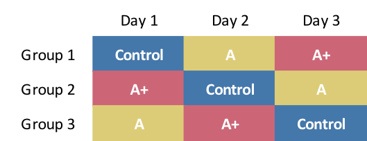
If we are free to assign any intervention on any day, one possible randomization scheme involving three interventions could look like this:

Key features of this scheme are: (1) all individuals are exposed to each intervention over three days, (2) on any given day, each intervention is applied to one group of participants (just in case the specific day has an impact on the outcome), and (3) not every permutation is included (for example, \(A\) does not immediately proceed \(Control\) in any sequence), because the relative ordering of interventions in this case is assumed not to matter. (We might need to expand to six groups to rectify this.)
Data simulation
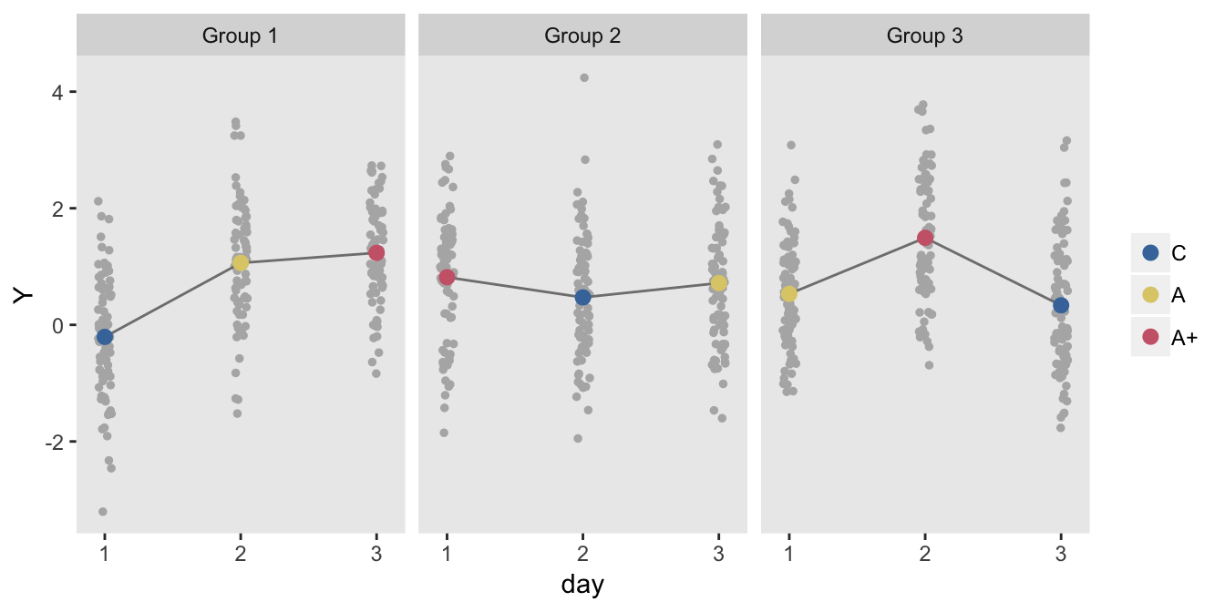
In this simulation, we will assume (1) that the outcome is slightly elevated on days two and three, (2) \(A\) is an improvement over \(Control\), (3) \(A^+\) is an improvement over \(A\), (4) there is strong correlation of outcomes within each individual, and (5) group membership has no bearing on the outcome.
First, I define the data, starting with the different sources of variation. I have specified a fairly high intra-class coefficient (ICC), because it is reasonable to assume that there will be quite a bit of variation across individuals:
vTotal = 1
vAcross <- iccRE(ICC = 0.5, varTotal = vTotal, "normal")
vWithin <- vTotal - vAcross

### Definitions

b <- defData(varname = "b", formula = 0, variance = vAcross,
             dist = "normal")

d <- defCondition(condition = "rxlab == 'C'",
       formula = "0 + b + (day == 2) * 0.5 + (day == 3) * 0.25",
       variance = vWithin, dist = "normal")
d <- defCondition(d, "rxlab == 'A'",
       formula = "0.4 + b + (day == 2) * 0.5 + (day == 3) * 0.25",
       variance = vWithin, dist = "normal")
d <- defCondition(d, "rxlab == 'A+'",
       formula = "1.0 + b + (day == 2) * 0.5 + (day == 3) * 0.25",
       variance = vWithin, dist = "normal")
Next, I generate the data, assigning three groups, each of which is tied to one of the three treatment sequences.
set.seed(39217)

db <- genData(240, b)
dd <- trtAssign(db, 3, grpName = "grp")
dd <- addPeriods(dd, 3)

dd[grp == 1, rxlab := c("C", "A", "A+")]
dd[grp == 2, rxlab := c("A+", "C", "A")]
dd[grp == 3, rxlab := c("A", "A+", "C")]

dd[, rxlab := factor(rxlab, levels = c("C", "A", "A+"))]
dd[, day := factor(period + 1)]

dd <- addCondition(d, dd, newvar = "Y")
dd
## timeID Y id period grp b rxlab day
## 1: 1 0.9015848 1 0 2 0.2664571 A+ 1
## 2: 2 1.2125919 1 1 2 0.2664571 C 2
## 3: 3 0.7578572 1 2 2 0.2664571 A 3
## 4: 4 2.0157066 2 0 3 1.1638244 A 1
## 5: 5 2.4948799 2 1 3 1.1638244 A+ 2
## ---
## 716: 716 1.9617832 239 1 1 0.3340201 A 2
## 717: 717 1.9231570 239 2 1 0.3340201 A+ 3
## 718: 718 1.0280355 240 0 3 1.4084395 A 1
## 719: 719 2.5021319 240 1 3 1.4084395 A+ 2
## 720: 720 0.4610550 240 2 3 1.4084395 C 3Here is a plot of the treatment averages each day for each of the three groups:
dm <- dd[, .(Y = mean(Y)), keyby = .(grp, period, rxlab)]
ngrps <- nrow(dm[, .N, keyby = grp])
nperiods <- nrow(dm[, .N, keyby = period])

ggplot(data = dm, aes(y=Y, x = period + 1)) +
  geom_jitter(data = dd, aes(y=Y, x = period + 1),
              width = .05, height = 0, color="grey70", size = 1 ) +
  geom_line(color = "grey50") +
  geom_point(aes(color = rxlab), size = 2.5) +
  scale_color_manual(values = c("#4477AA", "#DDCC77", "#CC6677")) +
  scale_x_continuous(name = "day", limits = c(0.9, nperiods + .1),
                     breaks=c(1:nperiods)) +
  facet_grid(~ factor(grp, labels = paste("Group", 1:ngrps))) +
  theme(panel.grid = element_blank(),
        legend.title = element_blank())
Estimating the effects
To estimate the treatment effects, I will use this mixed effects linear regression model:
\[Y_{it} = \alpha_0 + \gamma_{t} D_{it} + \beta_1 A_{it} + \beta_2 P_{it} + b_i + e_i\]
where \(Y_{it}\) is the outcome for individual \(i\) on day \(t\), \(t \in (1,2,3)\). \(A_{it}\) is an indicator for treatment \(A\) in time \(t\); likewise \(P_{it}\) is an indicator for \(A^+\). \(D_{it}\) is an indicator that the outcome was recorded on day \(t\). \(b_i\) is an individual (latent) random effect, \(b_i \sim N(0, \sigma_b^2)\). \(e_i\) is the (also latent) noise term, \(e_i \sim N(0, \sigma_e^2)\).
The parameter \(\alpha_0\) is the mean outcome on day 1 under \(Control\). The \(\gamma\)’s are the day-specific effects for days 2 and 3, with \(\gamma_1\) fixed at 0. \(\beta_1\) is the effect of \(A\) (relative to \(Control\)) and \(\beta_2\) is the effect of \(A^+\). In this case, the researchers were primarily interested in \(\beta_1\) and \(\beta_2 - \beta_1\), which is the incremental change from \(A\) to \(A^+\).
library(lme4)
lmerfit <- lmer(Y ~ day + rxlab + (1|id), data = dd)
rndTidy(lmerfit)
## term estimate std.error statistic group
## 1: (Intercept) -0.14 0.08 -1.81 fixed
## 2: day2 0.63 0.06 9.82 fixed
## 3: day3 0.38 0.06 5.97 fixed
## 4: rxlabA 0.57 0.06 8.92 fixed
## 5: rxlabA+ 0.98 0.06 15.35 fixed
## 6: sd_(Intercept).id 0.74 NA NA id
## 7: sd_Observation.Residual 0.70 NA NA ResidualAs to why we would want to bother with this complex design if we could just randomize individuals to one of three treatment groups, this little example using a more standard parallel design might provide a hint:
def2 <- defDataAdd(varname = "Y",
            formula = "0 + (frx == 'A') * 0.4 + (frx == 'A+') * 1",
            variance = 1, dist = "normal")

dd <- genData(240)
dd <- trtAssign(dd, nTrt = 3, grpName = "rx")

dd <- genFactor(dd, "rx", labels = c("C","A","A+"), replace = TRUE)
dd <- addColumns(def2, dd)

lmfit <- lm(Y~frx, data = dd)
rndTidy(lmfit)
## term estimate std.error statistic p.value
## 1: (Intercept) -0.12 0.10 -1.15 0.25
## 2: frxA 0.64 0.15 4.38 0.00
## 3: frxA+ 1.01 0.15 6.86 0.00If we compare the standard error for the effect of \(A^+\) in the two studies, the cross-over design is much more efficient (i.e. standard error is considerably smaller: 0.06 vs. 0.15). This really isn’t so surprising since we have collected a lot more data and modeled variation across individuals in the cross-over study.
Constrained cross-over design
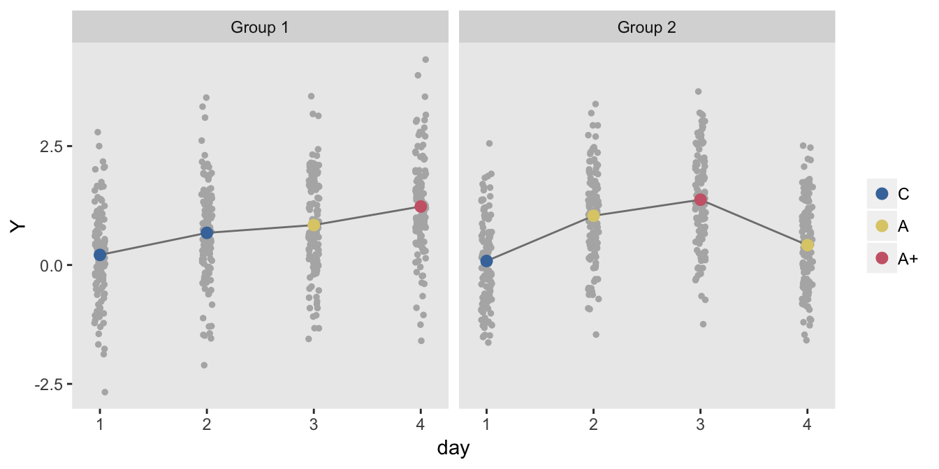
Unfortunately, the project was not at liberty to implement the three-way/three-day design just simulated. We came up with this approach that would provide some cross-over, but with an added day of treatment and measurement:

The data generation is slightly modified, though the original definitions can still be used:
db <- genData(240, b)
dd <- trtAssign(db, 2, grpName = "grp")
dd <- addPeriods(dd, 4)

dd[grp == 0, rxlab := c("C", "C", "A", "A+")]
dd[grp == 1, rxlab := c("C", "A", "A+", "A")]

dd[, rxlab := factor(rxlab, levels = c("C", "A", "A+"))]
dd[, day := factor(period + 1)]

dd <- addCondition(d, dd, "Y")
The model estimates indicate slightly higher standard errors than in the pure cross-over design:
lmerfit <- lmer(Y ~ day + rxlab + (1|id), data = dd)
rndTidy(lmerfit)
## term estimate std.error statistic group
## 1: (Intercept) 0.15 0.06 2.36 fixed
## 2: day2 0.48 0.08 6.02 fixed
## 3: day3 0.16 0.12 1.32 fixed
## 4: day4 -0.12 0.12 -1.02 fixed
## 5: rxlabA 0.46 0.10 4.70 fixed
## 6: rxlabA+ 1.14 0.12 9.76 fixed
## 7: sd_(Intercept).id 0.69 NA NA id
## 8: sd_Observation.Residual 0.68 NA NA ResidualHere are the key parameters of interest (refit using package lmerTest to get the contrasts). The confidence intervals include the true values (\(\beta_1 = 0.4\) and \(\beta_2 - \beta_1 = 0.6\)):
library(lmerTest)
lmerfit <- lmer(Y ~ day + rxlab + (1|id), data = dd)

L <- matrix(c(0, 0, 0, 0, 1, 0, 0, 0, 0, 0, -1, 1),
        nrow = 2, ncol = 6, byrow = TRUE)

con <- data.table(contest(lmerfit, L, confint = TRUE, joint = FALSE))
round(con[, .(Estimate, `Std. Error`, lower, upper)], 3)
## Estimate Std. Error lower upper
## 1: 0.462 0.098 0.269 0.655
## 2: 0.673 0.062 0.551 0.795Exploring bias
A single data set does not tell us if the proposed approach is indeed unbiased. Here, I generate 1000 data sets and fit the mixed effects model. In addition, I fit a model that ignores the day factor to see if it will induce bias (of course it will).
iter <- 1000
ests <- vector("list", iter)
xests <- vector("list", iter)

for (i in 1:iter) {

  db <- genData(240, b)
  dd <- trtAssign(db, 2, grpName = "grp")
  dd <- addPeriods(dd, 4)

  dd[grp == 0, rxlab := c("C", "C", "A", "A+")]
  dd[grp == 1, rxlab := c("C", "A", "A+", "A")]

  dd[, rxlab := factor(rxlab, levels = c("C", "A", "A+"))]
  dd[, day := factor(period + 1)]

  dd <- addCondition(d, dd, "Y")

  lmerfit <- lmer(Y ~ day + rxlab + (1|id), data = dd)
  xlmerfit <- lmer(Y ~ rxlab + (1|id), data = dd)

  ests[[i]] <- data.table(estA = fixef(lmerfit)[5],
      estAP = fixef(lmerfit)[6] - fixef(lmerfit)[5])

  xests[[i]] <-  data.table(estA = fixef(xlmerfit)[2],
      estAP = fixef(xlmerfit)[3] - fixef(xlmerfit)[2])

}

ests <- rbindlist(ests)
xests <- rbindlist(xests)
The results for the correct model estimation indicate that there is no bias (and that the standard error estimates from the model fit above were correct):
ests[, .(A.est =  round(mean(estA), 3),
         A.se =   round(sd(estA), 3),
         AP.est = round(mean(estAP), 3),
         AP.se =  round(sd(estAP), 3))]
## A.est A.se AP.est AP.se
## 1: 0.407 0.106 0.602 0.06In contrast, the estimates that ignore the day or period effect are in fact biased (as predicted):
xests[, .(A.est =  round(mean(estA), 3),
         A.se =   round(sd(estA), 3),
         AP.est = round(mean(estAP), 3),
         AP.se =  round(sd(estAP), 3))]
## A.est A.se AP.est AP.se
## 1: 0.489 0.053 0.474 0.057