Principled causal inference methods can be used to compare the effects of different exposures or treatments we have observed in non-experimental settings. These methods, which include matching (with or without propensity scores), inverse probability weighting, and various g-methods, help us create comparable groups to simulate a randomized experiment. All of these approaches rely on a key assumption of no unmeasured confounding. The problem is, short of subject matter knowledge, there is no way to test this assumption empirically.
The general approach to this problem has been to posit a level of unmeasured confounding that would be necessary to alter the conclusions of a study. The classic example (which also is probably the first) comes from the debate on the effects of smoking on lung cancer. There were some folks who argued that there was a genetic factor that was leading people to smoke and was simultaneously the cause of cancer. The great statistician Jerome Cornfield (who, I just saw on Wikipedia, happens to have shared my birthday), showed that an unobserved confounder (like a particular genetic factor) would need to lead to a 9-fold increase in the odds of smoking to explain away the association between smoking and cancer. Since such a strong factor was not likely to exist, he argued, the observed association was most likely real. (For a detailed discussion on various approaches to these kinds of sensitivity analyses, look at this paper by Liu, Kuramoto, and Stuart.)
My goal here is to think a bit more about what it means for a measured association to be sensitive to unmeasured confounding. When I originally started thinking about this, I thought that an association will be sensitive to unmeasured confounding if the underlying data generation process (DGP) actually includes an unmeasured confounder. Sure, if this is the case - that there actually is unmeasured confounding - then it is more likely that a finding will be sensitive to unmeasured confounding. But, this isn’t really that interesting, because we can’t observe the underlying DGP. And it is not necessarily the case that data sensitive to unmeasured confounding was in fact generated through some process with an unmeasured confounder.
Is there room for an alternative data generation process?
When considering sensitivity, it may be more useful to talk about the plausibility of alternative models. In this context, sensitivity is inherently related to the (1) the strength of the association of the observed exposure and outcome, and (2) the uncertainty (i.e. variability) around that association. Put succinctly, a relatively weak association with a lot of variability will be much more sensitive to unmeasured confounding than a strong association with little uncertainty. If you think in visual terms, when thinking about sensitivity, you might ask “do the data provide room for an alternative model?”
An alternative model
Let’s say we observe some exposure \(D\) and we are interested in its causal relationship with an outcome \(Y\), which we also observe. I am assuming \(D\) and \(Y\) are both continuous and normally distributed, which makes all of this work, but also limits how far I can take this. (To be more general, we will ultimately need more powerful tools, such as the R package treatSens, but more on that later.) Also, let’s assume for simplicity’s sake that there are no measured confounders - though that is not a requirement here.
With this observed data, we can go ahead and fit a simple linear regression model:
\[ Y = k_0 + k_1D,\] where \(k_1\) is the parameter of interest, the measured association of exposure \(D\) with the outcome \(Y\). (Again for simplicity, I am assuming \(k_1 > 0\).)
The question is, is there a possible underlying data generating process where \(D\) plays a minor role or none at all? For example, is there a possible DGP that looks like this:
\[ \begin{aligned} D &= \alpha_0 + \alpha_1 U + \epsilon_d \\ Y &= \beta_0 + \beta_1 D + \beta_2 U + \epsilon_y, \end{aligned} \]
where \(\beta_1 << k_1\), or perhaps \(\beta_1 = 0\)? That is, is there a process that generates the same observed distribution even though \(D\) is not a cause of \(Y\)? If so, how can we characterize that process, and is it plausible?
Simulation
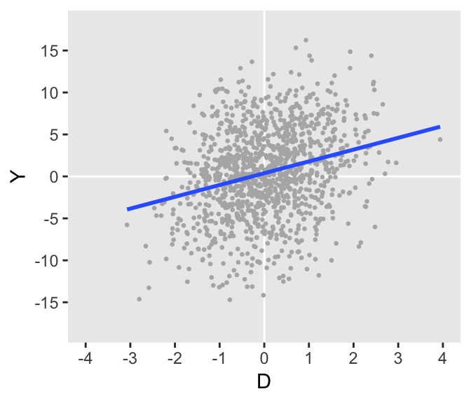
The observed DGP can be defined using simstudy. We can assume that the continuous exposure \(D\) can always be normalized (by centering and dividing by the standard deviation). In this example, the coefficients \(k_0 = 0\) and \(k_1 = 1.5\), so that a unit change in the normalized exposure leads, on average, to a positive change in \(Y\) of 1.5 units:
defO <- defData(varname = "D", formula = 0, variance = 1)
defO <- defData(defO, varname = "ey", formula = 0, variance = 25)
defO <- defData(defO, varname = "Y", formula = "1.5 * D + ey",
             dist = "nonrandom")
We can generate the data and take a look at it:
set.seed(20181201)
dtO <- genData(1200, defO)

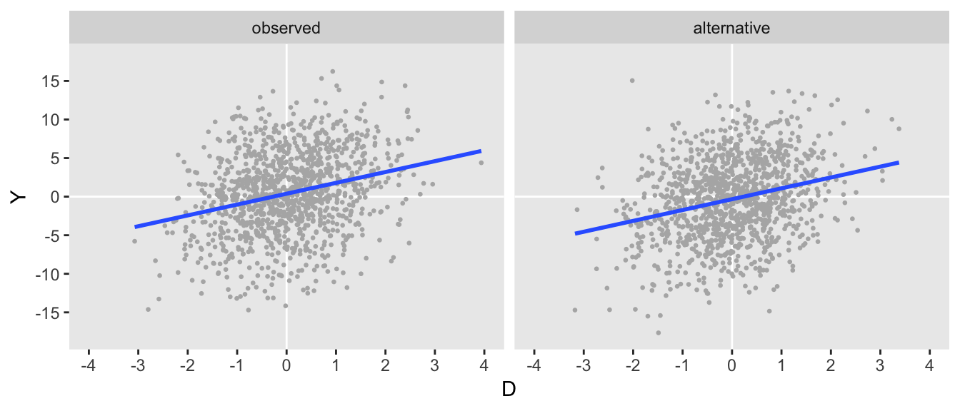
Can we specify another DGP that removes \(D\) from the process that defines \(Y\)? The answer in this case is “yes.” Here is one such example where both \(D\) and \(Y\) are a function of some unmeasured confounder \(U\), but \(Y\) is a function of \(U\) alone. The variance and coefficient specifications for this DGP may seem a bit arbitrary (and maybe even lucky), but how I arrived at these quantities will be the focus of the second part of this post, coming soon. (My real goal here is to pique your interest.)
defA1 <- defData(varname = "U", formula = 0, variance = 1)
defA1 <- defData(defA1, varname = "ed", formula = 0, variance = 0.727)
defA1 <- defData(defA1, varname = "D",  formula = "0.513 * U + ed",
              dist = "nonrandom")
defA1 <- defData(defA1, varname = "ey", formula = 0, variance = 20.412)
defA1 <- defData(defA1, varname = "Y", formula = "2.715 * U + ey",
              dist = "nonrandom")
After generating this second data set, we can see that they look pretty similar to each other:
set.seed(20181201)

dtO <- genData(1200, defO)
dtA1 <- genData(1200, defA1)
If the data are indeed similar, the covariance matrices generated by each of the data sets should also be similar, and they do appear to be:
dtO[, round(var(cbind(Y, D)), 1)]## Y D
## Y 27.8 1.4
## D 1.4 1.0dtA1[, round(var(cbind(Y, D)), 1)]## Y D
## Y 26.8 1.3
## D 1.3 1.0Non-unique data generating process
The DGP defined by defA1 is not a unique alternative. There are actually an infinite number of alternatives - here are two more, what I am calling “Alternative 2” and “Alternative 3” to go along with the first.
defA2 <- defData(varname = "U", formula = 0, variance = 1)
defA2 <- defData(defA2, varname = "ed", formula = 0, variance = 0.794)
defA2 <- defData(defA2, varname = "D",  formula = "0.444 * U + ed",
              dist = "nonrandom")
defA2 <- defData(defA2, varname = "ey", formula = 0, variance = 17.939)
defA2 <- defData(defA2, varname = "Y", formula = "3.138 * U + ey",
              dist = "nonrandom")
defA3 <- defData(varname = "U", formula = 0, variance = 1)
defA3 <- defData(defA3, varname = "ed", formula = 0, variance = 0.435)
defA3 <- defData(defA3, varname = "D", formula = "0.745 * U + ed",
dist = "nonrandom")
defA3 <- defData(defA3, varname = "ey", formula = 0, variance = 24.292)
defA3 <- defData(defA3, varname = "Y", formula = "1.869 * U + ey",
dist = "nonrandom")Rather than looking at plots of the four data sets generated by these equivalent processes, I fit four linear regression models based on the observed \(D\) and \(Y\). The parameter estimates and residual standard error estimates are quite close for all four:
| Observed | Alt 1 | Alt 2 | Alt 3 | |
| D | 1.41 | 1.41 | 1.41 | 1.37 |
| (0.15) | (0.15) | (0.15) | (0.15) | |
| Constant | 0.38 | -0.33 | -0.32 | -0.33 |
| (0.15) | (0.14) | (0.14) | (0.15) | |
| Residual Std. Error (df = 1198) | 5.08 | 4.99 | 4.98 | 5.02 |
Characterizing each data generation process
While each of the alternate DGPs lead to the same (or very similar) observed data distribution, the underlying relationships between \(U\), \(D\), and \(Y\) are quite different. In particular, if we inspect the correlations, we can see that they are quite different for each of the three alternatives. In fact, as you will see next time, all we need to do is specify a range of correlations for \(U\) and \(D\) to derive a curve that defines all the alternatives for a particular value of \(\beta_1\).
dtA1[, .(cor(U, D), cor(U, Y))]## V1 V2
## 1: 0.511 0.496dtA2[, .(cor(U, D), cor(U, Y))]## V1 V2
## 1: 0.441 0.579dtA3[, .(cor(U, D), cor(U, Y))]## V1 V2
## 1: 0.748 0.331Less sensitivity
So, what does it mean for an observed data set to be sensitive to unmeasured confounding? I would suggest that if an equivalent derived alternative DGP is based on “lower” correlations of \(U\) and \(D\) and/or \(U\) and \(Y\), then the observed data are more sensitive. What “low” correlation is will probably depend on the subject matter. I would say that the data we have been looking at above is moderately sensitive to unmeasured confounding.
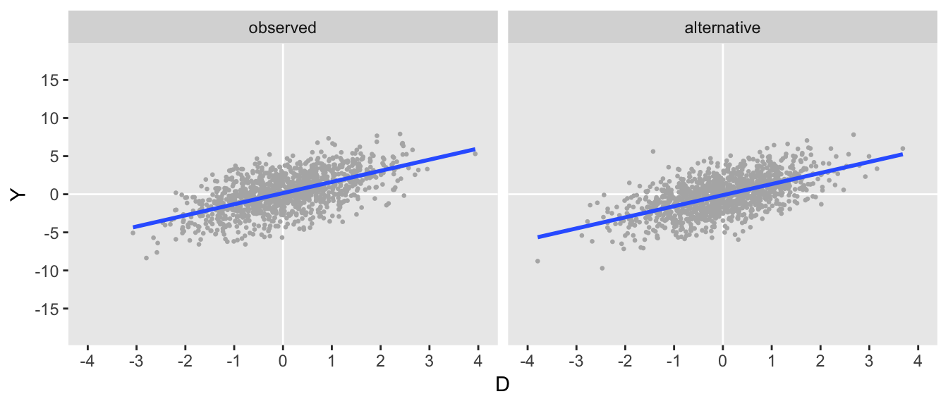
Here is an example of an observed data that might be considerably less sensitive:
defS <- updateDef(defO, changevar = "ey", newvariance = 4)

defAS <- defData(varname = "U", formula = 0, variance = 1)
defAS <- defData(defAS, varname = "ed", formula = 0, variance = 0.414)
defAS <- defData(defAS, varname = "D",  formula = "0.759 * U + ed",
              dist = "nonrandom")
defAS <- defData(defAS, varname = "ey", formula = 0, variance = 2.613)
defAS <- defData(defAS, varname = "Y", formula = "1.907 * U + ey",
              dist = "nonrandom")

set.seed(20181201)

dtS <- genData(1200, defS)
dtAS <- genData(1200, defAS)
The plots look similar, as do the covariance matrix describing the observed data:
dtS[, round(var(cbind(Y, D)), 1)]## Y D
## Y 6.3 1.4
## D 1.4 1.0dtAS[, round(var(cbind(Y, D)), 1)]## Y D
## Y 6.0 1.4
## D 1.4 1.0In this case, the both the correlations in the alternative DGP are quite high, suggesting a higher bar is needed to remove the association between \(D\) and \(Y\) entirely:
dtAS[, .(cor(U, D), cor(U, Y))]## V1 V2
## 1: 0.762 0.754In the second part of this post I will show how I derived the alternative DGPs, and then use that derivation to create an R function to generate sensitivity curves that allow us to visualize sensitivity in terms of the correlation parameters \(\rho_{UD}\) and \(\rho_{UY}\).