In my last post, I wrote about within- and between-period intra-cluster correlations in the context of stepped-wedge cluster randomized study designs. These are quite important to understand when figuring out sample size requirements (and models for analysis, which I’ll be writing about soon.) Here, I’m extending the constant ICC assumption I presented last time around by introducing some complexity into the correlation structure. Much of the code I am using can be found in last week’s post, so if anything seems a little unclear, hop over here.
Different within- and between-period ICC’s
In a scenario with constant within- and between-period ICC’s, the correlated data can be induced using a single cluster-level effect like \(b_c\) in this model:
\[ Y_{ict} = \mu + \beta_0t + \beta_1X_{ct} + b_{c} + e_{ict} \]
More complexity can be added if, instead of a single cluster level effect, we have a vector of correlated cluster/time specific effects \(\mathbf{b_c}\). These cluster-specific random effects \((b_{c1}, b_{c2}, \ldots, b_{cT})\) replace \(b_c\), and the slightly modified data generating model is
\[ Y_{ict} = \mu + \beta_0t + \beta_1X_{ct} + b_{ct} + e_{ict} \]
The vector \(\mathbf{b_c}\) has a multivariate normal distribution \(N_T(0, \sigma^2_b \mathbf{R})\). This model assumes a common covariance structure across all clusters, \(\sigma^2_b \mathbf{R}\), where the general version of \(\mathbf{R}\) is
\[ \mathbf{R} = \left( \begin{matrix} 1 & r_{12} & r_{13} & \cdots & r_{1T} \\ r_{21} & 1 & r_{23} & \cdots & r_{2T} \\ r_{31} & r_{32} & 1 & \cdots & r_{3T} \\ \vdots & \vdots & \vdots & \vdots & \vdots \\ r_{T1} & r_{T2} & r_{T3} & \cdots & 1 \end{matrix} \right ) \]
Within-period cluster correlation
The covariance of any two individuals \(i\) and \(j\) in the same cluster \(c\) and same period \(t\) is
\[ \begin{aligned} cov(Y_{ict}, Y_{jct}) &= cor(\mu + \beta_0t + \beta_1X_{ct} + b_{ct} + e_{ict}, \ \mu + \beta_0t + \beta_1X_{ct} + b_{ct} + e_{jct}) \\ \\ &= cov(b_{ct}, b_{ct}) + cov(e_{ict}, e_{jct}) \\ \\ &=var(b_{ct}) + 0 \\ \\ &= \sigma^2_b r_{tt} \\ \\ &= \sigma^2_b \qquad \qquad \qquad \text{since } r_{tt} = 1, \ \forall t \in \ ( 1, \ldots, T) \end{aligned} \]
And I showed in the previous post that \(var(Y_{ict}) = var(Y_{jct}) = \sigma^2_b + \sigma^2_e\), so the within-period intra-cluster correlation is what we saw last time:
\[ICC_{tt} = \frac{\sigma^2_b}{\sigma^2_b+\sigma^2_e}\]
Between-period cluster correlation
The covariance of any two individuals in the same cluster but two different time periods \(t\) and \(t^{\prime}\) is:
\[ \begin{aligned} cov(Y_{ict}, Y_{jct^{\prime}}) &= cor(\mu + \beta_0t + \beta_1X_{ct} + b_{ct} + e_{ict}, \ \mu + \beta_0t + \beta_1X_{ct^{\prime}} + b_{ct^{\prime}} + e_{jct^{\prime}}) \\ \\ &= cov(b_{ct}, b_{ct^{\prime}}) + cov(e_{ict}, e_{jct^{\prime}}) \\ \\ &= \sigma^2_br_{tt^{\prime}} \end{aligned} \]
Based on this, the between-period intra-cluster correlation is
\[ ICC_{tt^\prime} =\frac{\sigma^2_b}{\sigma^2_b+\sigma^2_e} r_{tt^{\prime}}\]
Adding structure to matrix \(\mathbf{R}\)
This paper by Kasza et al, which describes various stepped-wedge models, suggests a structured variation of \(\mathbf{R}\) that is a function of two parameters, \(r_0\) and \(r\):
\[ \mathbf{R} = \mathbf{R}(r_0, r) = \left( \begin{matrix} 1 & r_0r & r_0r^2 & \cdots & r_0r^{T-1} \\ r_0r & 1 & r_0 r & \cdots & r_0 r^{T-2} \\ r_0r^2 & r_0 r & 1 & \cdots & r_0 r^{T-3} \\ \vdots & \vdots & \vdots & \vdots & \vdots \\ r_0r^{T-1} & r_0r^{T-2} & r_0 r^{T-3} & \cdots & 1 \end{matrix} \right ) \]
How we specify \(r_0\) and \(r\) reflects different assumptions about the between-period intra-cluster correlations. I describe two particular cases below.
Constant correlation over time
In this first case, the correlation between individuals in the same cluster but different time periods is less than the correlation between individuals in the same cluster and same time period. In other words, \(ICC_{tt} \ne ICC_{tt^\prime}\). However the between-period correlation is constant, or \(ICC_{tt^\prime}\) are constant for all \(t\) and \(t^\prime\). We have these correlations when \(r_0 = \rho\) and \(r = 1\), giving
\[ \mathbf{R} = \mathbf{R}(\rho, 1) = \left( \begin{matrix} 1 & \rho & \rho & \cdots & \rho \\ \rho & 1 & \rho & \cdots & \rho \\ \rho & \rho & 1 & \cdots & \rho \\ \vdots & \vdots & \vdots & \vdots & \vdots \\ \rho & \rho & \rho & \cdots & 1 \end{matrix} \right ) \]
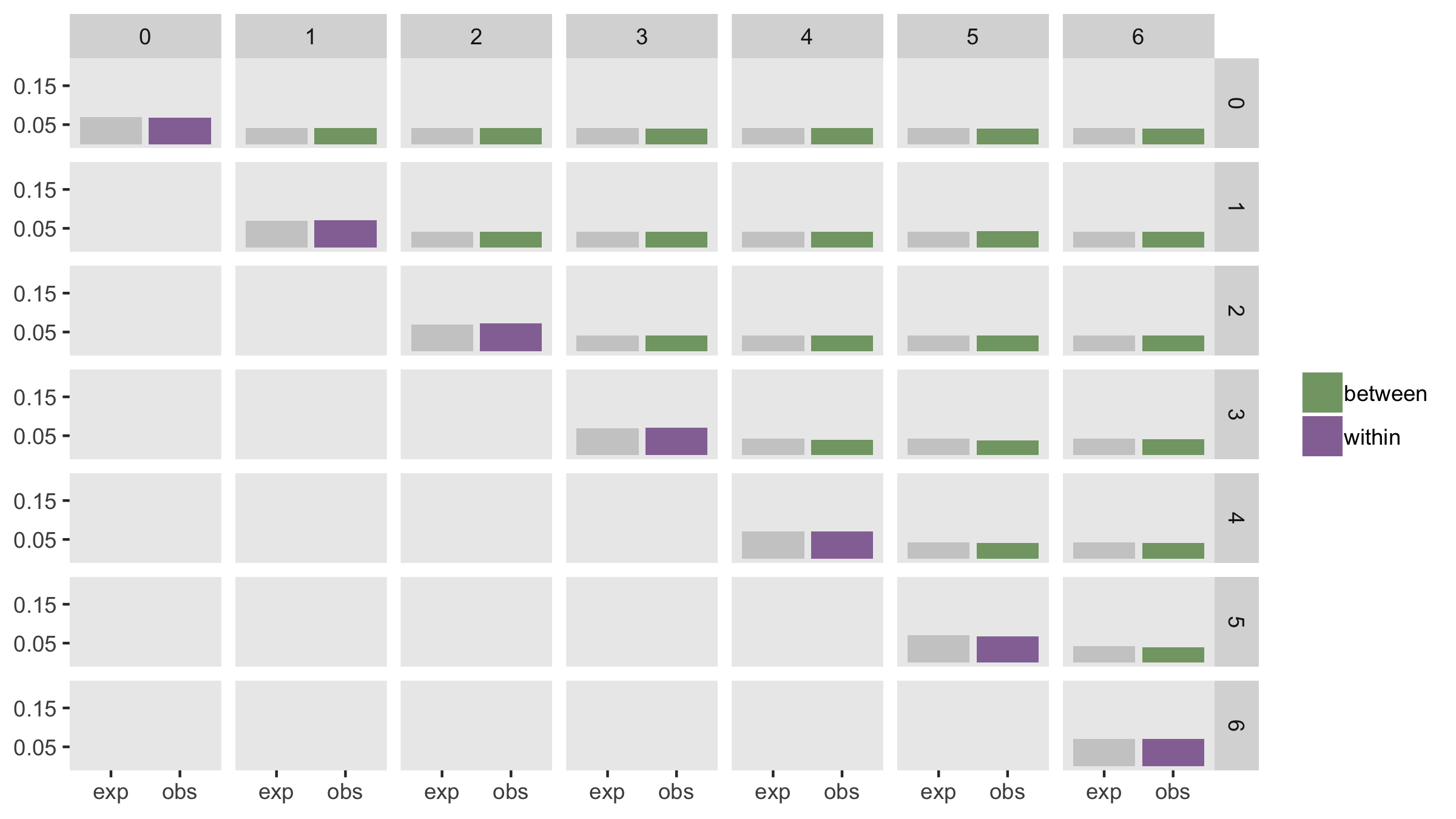
To simulate under this scenario, I am setting \(\sigma_b^2 = 0.15\), \(\sigma_e^2 = 2.0\), and \(\rho = 0.6\). We would expect the following ICC’s:
\[ \begin{aligned} ICC_{tt} &= \frac{0.15}{0.15+2.00} = 0.0698 \\ \\ ICC_{tt^\prime} &= \frac{0.15}{0.15+2.00}\times0.6 = 0.0419 \end{aligned} \]
Here is the code to define and generate the data:
defc <- defData(varname = "mu", formula = 0,
                dist = "nonrandom", id = "cluster")
defc <- defData(defc, "s2", formula = 0.15, dist = "nonrandom")

defa <- defDataAdd(varname = "Y",
                   formula = "0 + 0.10  * period + 1 * rx + cteffect",
                   variance = 2, dist = "normal")

dc <- genData(100, defc)
dp <- addPeriods(dc, 7, "cluster")
dp <- trtStepWedge(dp, "cluster", nWaves = 4, lenWaves = 1, startPer = 2)
dp <- addCorGen(dtOld = dp, nvars = 7, idvar = "cluster",
                rho = 0.6, corstr = "cs", dist = "normal",
                param1 = "mu", param2 = "s2", cnames = "cteffect")

dd <- genCluster(dp, cLevelVar = "timeID", numIndsVar = 100,
                 level1ID = "id")
dd <- addColumns(defa, dd)
As I did in my previous post, I’ve generated 200 data sets, estimated the within- and between-period ICC’s for each data set, and computed the average for each. The plot below shows the expected values in gray and the estimated values in purple and green.

Declining correlation over time
In this second case, we make an assumption that the correlation between individuals in the same cluster degrades over time. Here, the correlation between two individuals in adjacent time periods is stronger than the correlation between individuals in periods further apart. That is \(ICC_{tt^\prime} > ICC_{tt^{\prime\prime}}\) if \(|t^\prime - t| < |t^{\prime\prime} - t|\). This structure can be created by setting \(r_0 = 1\) and \(r=\rho\), giving us an auto-regressive correlation matrix \(R\):
\[ \mathbf{R} = \mathbf{R}(1, \rho) = \left( \begin{matrix} 1 & \rho & \rho^2 & \cdots & \rho^{T-1} \\ \rho & 1 & \rho & \cdots & \rho^{T-2} \\ \rho^2 & \rho & 1 & \cdots & \rho^{T-3} \\ \vdots & \vdots & \vdots & \vdots & \vdots \\ \rho^{T-1} & \rho^{T-2} & \rho^{T-3} & \cdots & 1 \end{matrix} \right ) \]
I’ve generated data using the same variance assumptions as above. The only difference in this case is that the corstr argument in the call to addCorGen is “ar1” rather than “cs” (which was used above). Here are a few of the expected correlations:
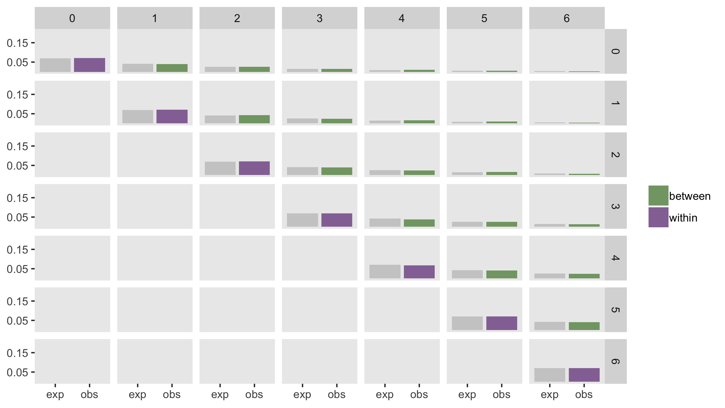
\[ \begin{aligned} ICC_{t,t} &= \frac{0.15}{0.15+2.00} = 0.0698 \\ \\ ICC_{t,t+1} &= \frac{0.15}{0.15+2.00}\times 0.6^{1} = 0.0419 \\ \\ ICC_{t,t+2} &= \frac{0.15}{0.15+2.00}\times 0.6^{2} = 0.0251 \\ \\ \vdots \\ ICC_{t, t+6} &= \frac{0.15}{0.15+2.00}\times 0.6^{6} = 0.0032 \end{aligned} \]
And here is the code:
defc <- defData(varname = "mu", formula = 0,
                dist = "nonrandom", id = "cluster")
defc <- defData(defc, "s2", formula = 0.15, dist = "nonrandom")

defa <- defDataAdd(varname = "Y",
                   formula = "0 + 0.10  * period + 1 * rx + cteffect",
                   variance = 2, dist = "normal")

dc <- genData(100, defc)
dp <- addPeriods(dc, 7, "cluster")
dp <- trtStepWedge(dp, "cluster", nWaves = 4, lenWaves = 1, startPer = 2)
dp <- addCorGen(dtOld = dp, nvars = 7, idvar = "cluster",
                rho = 0.6, corstr = "ar1", dist = "normal",
                param1 = "mu", param2 = "s2", cnames = "cteffect")

dd <- genCluster(dp, cLevelVar = "timeID", numIndsVar = 10,
                 level1ID = "id")
dd <- addColumns(defa, dd)
And here are the observed average estimates (based on 200 datasets) alongside the expected values:

Random slope
In this last case, I am exploring what the ICC’s look like in the context of random effects model that includes a cluster-specific intercept \(b_c\) and a cluster-specific slope \(s_c\):
\[ Y_{ict} = \mu + \beta_0 t + \beta_1 X_{ct} + b_c + s_c t + e_{ict} \]
Both \(b_c\) and \(s_c\) are normally distributed with mean 0, and variances \(\sigma_b^2\) and \(\sigma_s^2\), respectively. (In this example \(\sigma_b^2\) and \(\sigma_s^2\) are uncorrelated, but that may not necessarily be the case.)
Because of the random slopes, the variance of the \(Y\)’s increase over time:
\[ var(Y_{ict}) = \sigma^2_b + t^2 \sigma^2_s + \sigma^2_e \]
The same is true for the within- and between-period covariances:
\[ \begin{aligned} cov(Y_{ict}, Y_{jct}) &= \sigma^2_b + t^2 \sigma^2_s \\ \\ cov(Y_{ict}, Y_{jct^\prime}) &= \sigma^2_b + tt^\prime \sigma^2_s \\ \end{aligned} \]
The ICC’s that follow from these various variances and covariances are:
\[ \begin{aligned} ITT_{tt} &= \frac{\sigma^2_b + t^2 \sigma^2_s}{\sigma^2_b + t^2 \sigma^2_s + \sigma^2_e}\\ \\ ITT_{tt^\prime} & = \frac{\sigma^2_b + tt^\prime \sigma^2_s}{\left[(\sigma^2_b + t^2 \sigma^2_s + \sigma^2_e)(\sigma^2_b + {t^\prime}^2 \sigma^2_s + \sigma^2_e)\right]^\frac{1}{2}} \end{aligned} \]
In this example, \(\sigma^2_s = 0.01\) (and the other variances remain as before), so
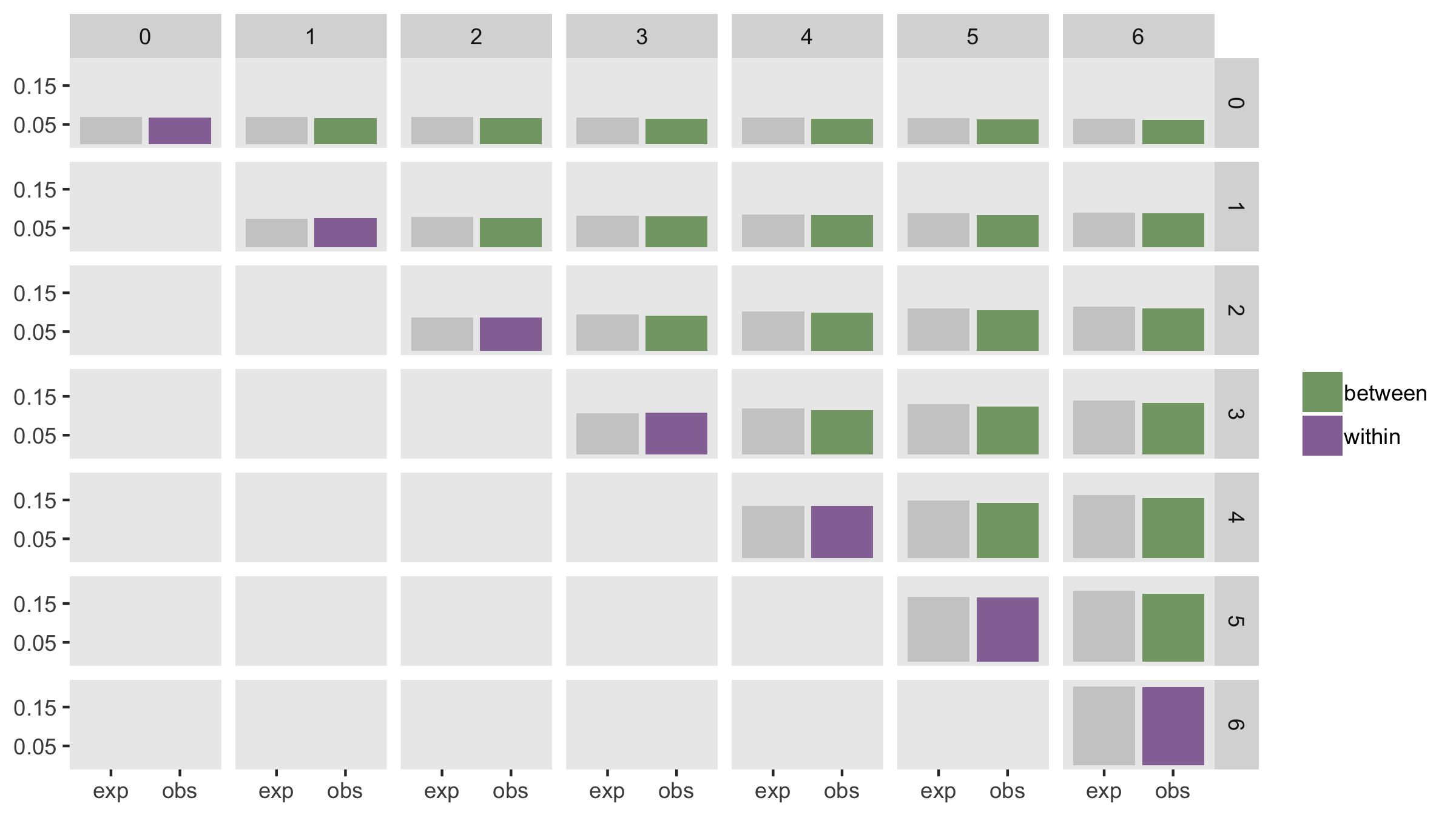
\[ ITT_{33} = \frac{0.15 + 3^2 \times 0.01}{0.15 + 3^2 \times 0.01 + 2} =0.1071\] and
\[ ITT_{36} = \frac{0.15 + 3 \times 6 \times 0.01}{\left[(0.15 + 3^2 \times 0.01 + 2)(0.15 + 6^2 \times 0.01 + 2)\right ]^\frac{1}{2}} =0.1392\]
Here’s the data generation:
defc <- defData(varname = "ceffect", formula = 0, variance = 0.15,
                dist = "normal", id = "cluster")
defc <- defData(defc, "cteffect", formula = 0, variance = 0.01,
                dist = "normal")

defa <- defDataAdd(varname = "Y",
  formula = "0 + ceffect + 0.10  * period + cteffect * period + 1 * rx",
  variance = 2, dist = "normal")

dc <- genData(100, defc)
dp <- addPeriods(dc, 7, "cluster")
dp <- trtStepWedge(dp, "cluster", nWaves = 4, lenWaves = 1, startPer = 2)

dd <- genCluster(dp, cLevelVar = "timeID", numIndsVar = 10,
                 level1ID = "id")
dd <- addColumns(defa, dd)
And here is the comparison between observed and expected ICC’s. The estimates are quite variable, so there appears to be slight bias. However, if I generated more than 200 data sets, the mean would likely converge closer to the expected values.

In the next post (or two), I plan on providing some examples of fitting models to the data I’ve generated here. In some cases, fairly standard linear mixed effects models in R may be adequate, but in others, we may need to look elsewhere.
References:
Kasza, J., K. Hemming, R. Hooper, J. N. S. Matthews, and A. B. Forbes. “Impact of non-uniform correlation structure on sample size and power in multiple-period cluster randomised trials.” Statistical methods in medical research (2017): 0962280217734981.