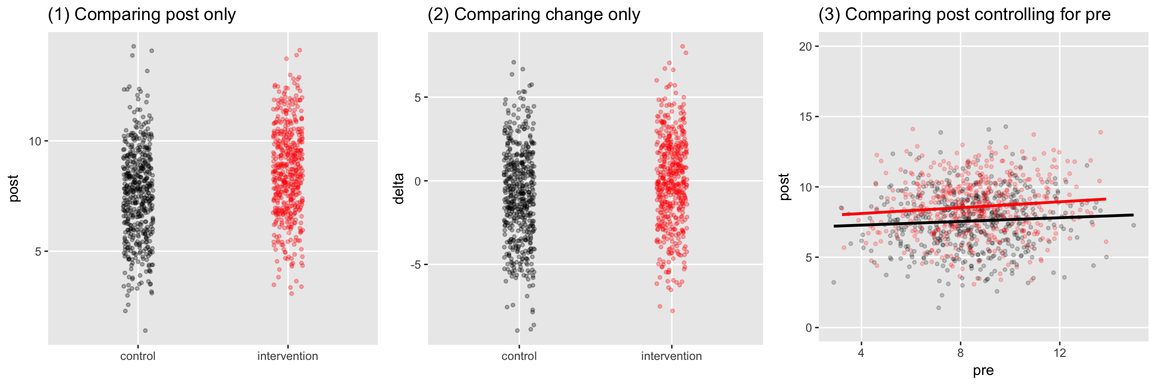
Well, maybe you haven’t, but this seems to come up all the time. An investigator wants to assess the effect of an intervention on a outcome. Study participants are randomized either to receive the intervention (could be a new drug, new protocol, behavioral intervention, whatever) or treatment as usual. For each participant, the outcome measure is recorded at baseline - this is the pre in pre/post analysis. The intervention is delivered (or not, in the case of the control group), some time passes, and the outcome is measured a second time. This is our post. The question is, how should we analyze this study to draw conclusions about the intervention’s effect on the outcome?
There are at least three possible ways to approach this. (1) Ignore the pre outcome measure and just compare the average post scores of the two groups. (2) Calculate a change score for each individual (Δi=posti−prei), and compare the average Δ’s for each group. Or (3), use a more sophisticated regression model to estimate the intervention effect while controlling for the pre or baseline measure of the outcome. Here are three models associated with each approach (Ti is 1 if the individual i received the treatment, 0 if not, and ϵi is an error term):
(1) posti=β0+β1Ti+ϵi(2) Δi=α0+α1Ti+ϵi(3) posti=γ0+γ1prei+γ2Ti+ϵi
I’ve explored various scenarios (i.e. different data generating assumptions) to see if it matters which approach we use. (Of course it does.)
Scenario 1: pre and post not correlated
In the simulations that follow, I am generating potential outcomes for each individual. So, the variable post0 represents the follow-up outcome for the individual under the control condition, and post1 is the outcome in the intervention condition. pre0 and pre1 are the same, because the intervention does not affect the baseline measurement. The effect of the intervention is specified by eff. In the first scenario, the baseline and follow-up measures are not related to each other, and the effect size is 1. All of the data definitions and data generation are done using package simstudy.
library(simstudy)
defPO <- defData(varname = "pre0", formula = 8.5,
variance = 4, dist = "normal")
defPO <- defData(defPO, varname = "post0", formula = 7.5,
variance = 4, dist = "normal")
defPO <- defData(defPO, varname = "pre1", formula = "pre0",
dist = "nonrandom")
defPO <- defData(defPO, varname = "eff", formula = 1,
variance = 0.2, dist = "normal")
defPO <- defData(defPO, varname = "post1", formula = "post0 + eff",
dist = "nonrandom")
The baseline, follow-up, and change that are actually observed are merely a function of the group assignment.
defObs <- defDataAdd(varname = "pre",
formula = "pre0 * (trtGrp == 0) + pre1 * (trtGrp == 1)",
dist = "nonrandom")
defObs <- defDataAdd(defObs, varname = "post",
formula = "post0 * (trtGrp == 0) + post1 * (trtGrp == 1)",
dist = "nonrandom")
defObs <- defDataAdd(defObs, varname = "delta",
formula = "post - pre",
dist = "nonrandom")
Now we generate the potential outcomes, the group assignment, and observed data for 1000 individuals. (I’m using package stargazer, definitely worth checking out, to print out the first five rows of the dataset.)
set.seed(123)

dt <- genData(1000, defPO)
dt <- trtAssign(dt)
dt <- addColumns(defObs, dt)

stargazer::stargazer(dt[1:5,], type = "text", summary=FALSE, digits = 2)
##
## =========================================================
##   id trtGrp pre0  post0 pre1  eff  post1  pre  post delta
## ---------------------------------------------------------
## 1 1    1    7.38  5.51  7.38  0.77 6.28  7.38  6.28 -1.10
## 2 2    1    8.04  5.42  8.04  1.11 6.53  8.04  6.53 -1.51
## 3 3    1    11.62 7.46  11.62 0.76 8.22  11.62 8.22 -3.40
## 4 4    0    8.64  7.24  8.64  1.55 8.78  8.64  7.24 -1.41
## 5 5    1    8.76  2.40  8.76  1.08 3.48  8.76  3.48 -5.28
## ---------------------------------------------------------
The plots show the three different types of analysis - follow-up measurement alone, change, or follow-up controlling for baseline:

I compare the different modeling approaches by using simulation to estimate statistical power for each. That is, given that there is some effect, how often is the p-value of the test less than 0.05. I’ve written a function to handle the data generation and power estimation. The function generates 1000 data sets of a specified sample size, each time fitting the three models, and keeping track of the relevant p-values for each iteration.
powerFunc <- function(def, addDef, ss, rct = TRUE) {

  presults <- data.table()
  iter <- 1000

  for (i in 1:iter) {

    dt <- genData(ss, def)

    if (rct) {
      dt <- trtAssign(dt)
    } else {
      dt <- trtObserve(dt, "-4.5 + .5*pre0", logit.link = TRUE)
    }

    dt <- addColumns(addDef, dt)

    lmfit1 <- lm(post ~ trtGrp, data = dt)
    lmfit2 <- lm(delta ~ trtGrp, data = dt)
    lmfit3 <- lm(post ~ pre + trtGrp, data = dt)
    lmfit3x <- lm(post ~ pre + trtGrp + pre*trtGrp, data = dt)

    p1 <- coef(summary(lmfit1))["trtGrp","Pr(>|t|)" ]
    p2 <- coef(summary(lmfit2))["trtGrp","Pr(>|t|)" ]
    p3 <- coef(summary(lmfit3))["trtGrp","Pr(>|t|)" ]
    p3x <- coef(summary(lmfit3x))["pre:trtGrp","Pr(>|t|)" ]

    presults <- rbind(presults, data.table(p1, p2, p3, p3x))
  }

  return(presults)

}
The results for the first data set are based on a sample size of 150 individuals (75 in each group). The post-only model does just as well as the post adjusted for baseline model. The model evaluating change in this scenario is way under powered.
presults <- powerFunc(defPO, defObs, 150)

presults[, .(postonly = mean(p1 <= 0.05),
             change = mean(p2 <= 0.05),
             adjusted = mean(p3 <= 0.05))]
##    postonly change adjusted
## 1:     0.85  0.543    0.845
Scenario 2: pre and post are moderately correlated
Now, we update the definition of post0 so that it is now a function of pre0, so that the correlation is around 0.45.
defPO <- updateDef(defPO, changevar = "post0",
                 newformula = "3.5 + 0.47 * pre0",
                 newvariance = 3)

The correlation actually increases power, so we use a reduced sample size of 120 for the power estimation. In this case, the three models actually all do pretty well, but the adjusted model is slightly superior.
##    postonly change adjusted
## 1:    0.776  0.771    0.869
Scenario 3: pre and post are almost perfectly correlated
When baseline and follow-up measurements are almost perfectly correlated (in this case about 0.85), we would be indifferent between the change and adjusted analyses - the power of the tests is virtually identical. However, the analysis that considers the follow-up measure alone does is much less adequate, due primarily to the measure’s relatively high variability.
defPO <- updateDef(defPO, changevar = "post0",
                 newformula = "0.9 * pre0",
                 newvariance = 1)

##    postonly change adjusted
## 1:    0.358  0.898    0.894
When the effect differs by baseline measurement
In a slight variation of the previous scenario, the effect of the intervention itself is a now function of the baseline score. Those who score higher will benefit less from the intervention - they simply have less room to improve. In this case, the adjusted model appears slightly inferior to the change model, while the unadjusted post-only model is still relatively low powered.
defPO <- updateDef(defPO, changevar = "eff",
                 newformula = "1.9 - 1.9 * pre0/15")

presults[, .(postonly = mean(p1 <= 0.05),
             change = mean(p2 <= 0.05),
             adjusted = mean(p3 <= 0.025 | p3x <= 0.025))]
##    postonly change adjusted
## 1:    0.425  0.878    0.863
The adjusted model has less power than the change model, because I used a reduced α-level for the hypothesis test of the adjusted models. I am testing for interaction first, then if that fails, for main effects, so I need to adjust for multiple comparisons. (I have another post that shows why this might be a good thing to do.) I have used a Bonferroni adjustment, which can be a more conservative test. I still prefer the adjusted model, because it provides more insight into the underlying process than the change model.
Treatment assignment depends on baseline measurement
Now, slightly off-topic. So far, we’ve been talking about situations where treatment assignment is randomized. What happens in a scenario where those with higher baseline scores are more likely to receive the intervention? Well, if we don’t adjust for the baseline score, we will have unmeasured confounding. A comparison of follow-up scores in the two groups will be biased towards the intervention group if the baseline scores are correlated with follow-up scores - as we see visually with a scenario in which the effect size is set to 0. Also notice that the p-values for the unadjusted model are consistently below 0.05 - we are almost always drawing the wrong conclusion if we use this model. On the other hand, the error rate for the adjusted model is close to 0.05, what we would expect.
defPO <- updateDef(defPO, changevar = "eff",
                 newformula = 0)

dt <- genData(1000, defPO)
dt <- trtObserve(dt, "-4.5 + 0.5 * pre0", logit.link = TRUE)
dt <- addColumns(defObs, dt)

##    postonly change adjusted
## 1:    0.872  0.095    0.046
I haven’t proved anything here, but these simulations suggest that we should certainly think twice about using an unadjusted model if we happen to have baseline measurements. And it seems like you are likely to maximize power (and maybe minimize bias) if you compare follow-up scores while adjusting for baseline scores rather than analyzing change in scores by group.


