I recently described why we might want to conduct a multi-factorial experiment, and I alluded to the fact that this approach can be quite efficient. It is efficient in the sense that it is possible to test simultaneously the impact of multiple interventions using an overall sample size that would be required to test a single intervention in a more traditional RCT. I demonstrate that here, first with a continuous outcome and then with a binary outcome.
In all of the examples that follow, I am assuming we are in an exploratory phase of research, so our alpha levels are relaxed a bit to . In addition, we make no adjustments for multiple testing. This might be justifiable, since we are not as concerned about making a Type 1 error (concluding an effect is real when there isn’t actually one). Because this is a screening exercise, the selected interventions will be re-evaluated. At the same time, we are setting desired power to be 90%. This way, if an effect really exists, we are more likely to select it for further review.
Two scenarios with a continuous outcome
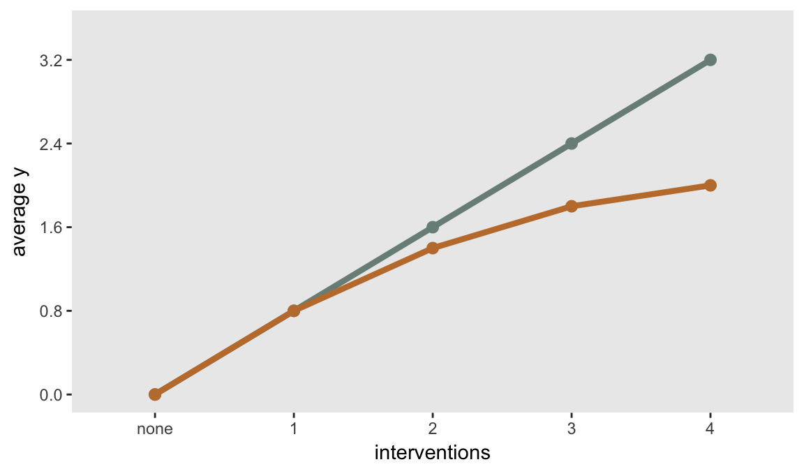
To start, I have created two sets of underlying assumptions. In the first, the effects of the four interventions (labeled fac1, fac2, fac3, and fac4) are additive. (The factor variables are parameterized using effect-style notation, where the value -1 represents no intervention and 1 represents the intervention.) So, with no interventions the outcome is 0, and each successive intervention adds 0.8 to the observed outcome (on average), so that individuals exposed to all four factors will have an average outcome .
cNoX <- defReadCond("DataMF/FacSumContNoX.csv")
cNoX
## condition formula variance dist link
## 1: (fac1 + fac2 + fac3 + fac4) == -4 0.0 9.3 normal identity
## 2: (fac1 + fac2 + fac3 + fac4) == -2 0.8 9.3 normal identity
## 3: (fac1 + fac2 + fac3 + fac4) == 0 1.6 9.3 normal identity
## 4: (fac1 + fac2 + fac3 + fac4) == 2 2.4 9.3 normal identity
## 5: (fac1 + fac2 + fac3 + fac4) == 4 3.2 9.3 normal identityIn the second scenario, each successive exposure continues to add to the effect, but each additional intervention adds a little less. The first intervention adds 0.8, the second adds 0.6, the third adds 0.4, and the fourth adds 0.2. This is a form of interaction.
cX <- defReadCond("DataMF/FacSumContX.csv")
cX
## condition formula variance dist link
## 1: (fac1 + fac2 + fac3 + fac4) == -4 0.0 9.3 normal identity
## 2: (fac1 + fac2 + fac3 + fac4) == -2 0.8 9.3 normal identity
## 3: (fac1 + fac2 + fac3 + fac4) == 0 1.4 9.3 normal identity
## 4: (fac1 + fac2 + fac3 + fac4) == 2 1.8 9.3 normal identity
## 5: (fac1 + fac2 + fac3 + fac4) == 4 2.0 9.3 normal identityThis is what a plot of the means might look like for each of the scenarios. The straight line represents the additive (non-interactive) scenario, and the bent line is the interaction scenario:

Sample size requirement for a single intervention compared to control
If we were to conduct a more traditional randomized experiment with two groups - treatment and control - we would need about 500 total subjects under the assumptions that we are using:
power.t.test(power = 0.90, delta = .8, sd = 3.05, sig.level = 0.10)##
## Two-sample t test power calculation
##
## n = 249.633
## delta = 0.8
## sd = 3.05
## sig.level = 0.1
## power = 0.9
## alternative = two.sided
##
## NOTE: n is number in *each* groupTo take a look at the sample size requirements for a multi-factorial study, I’ve written this function that repeatedly samples data based on the definitions and fits the appropriate model, storing the results after each model estimation.
library(simstudy)

iterFunc <- function(dc, dt, seed = 464653, iter = 1000, binary = FALSE) {

  set.seed(seed)
  res <- list()

  for (i in 1:iter) {

    dx <- addCondition(dc, dt, "Y")

    if (binary == FALSE) {
      fit <- lm(Y~fac1*fac2*fac3*fac4, data = dx)
    } else {
      fit <- glm(Y~fac1*fac2*fac3*fac4, data = dx, family = binomial)
    }

    # A simple function to pull data from the fit

    res <- appendRes(res, fit)

  }

  return(res)
}
And finally, here are the results for the sample size requirements based on no interaction across interventions. (I am using function genMultiFac to generate replications of all the combinations of four factors. This function is now part of simstudy, which is available on github, and will hopefully soon be up on CRAN.)
dt <- genMultiFac(32, nFactors = 4, coding = "effect",
                  colNames = paste0("fac", c(1:4)))

res <- iterFunc(cNoX, dt)
apply(res$p[, .(fac1, fac2, fac3, fac4)] < 0.10, 2, mean)## fac1 fac2 fac3 fac4
## 0.894 0.895 0.905 0.902A sample size of gives us 90% power that we are seeking. In case you don’t believe my simulation, we can compare the estimate provided by the MOST package, created by the Methodology Center at Penn State:
library(MOST)
FactorialPowerPlan(alpha = 0.10, model_order = 1, nfactors = 4,
                   ntotal = 500, sigma_y = 3.05, raw_main = 0.8)$power
## [1] "------------------------------------------------------------"
## [1] "FactorialPowerPlan Macro"
## [1] "The Methodology Center"
## [1] "(c) 2012 Pennsylvania State University"
## [1] "------------------------------------------------------------"
## [1] "Assumptions:"
## [1] "There are 4 dichotomous factors."
## [1] "There is independent random assignment."
## [1] "Analysis will be based on main effects only."
## [1] "Two-sided alpha: 0.10"
## [1] "Total number of participants: 500"
## [1] "Effect size as unstandardized difference in means: 0.80"
## [1] "Assumed standard deviation for the response variable is 3.05"
## [1] "Attempting to calculate the estimated power."
## [1] "------------------------------------------------------------"
## [1] "Results:"
## [1] "The calculated power is 0.9004"## [1] 0.9004Interaction
A major advantage of the multi-factorial experiment over the traditional RCT, of course, is that it allows us to investigate if the interventions interact in any interesting ways. However, in practice it may be difficult to generate sample sizes large enough to measure these interactions with much precision.
In the next pair of simulations, we see that even if we are only interested in exploring the main effects, underlying interaction reduces power. If there is actually interaction (as in the second scenario defined above), the original sample size of 500 may be inadequate to estimate the main effects:
dt <- genMultiFac(31, nFactors = 4, coding = "effect",
                  colNames = paste0("fac", c(1:4)))

res <- iterFunc(cX, dt)

apply(res$p[, .(fac1, fac2, fac3, fac4)] < 0.10, 2, mean)
## fac1 fac2 fac3 fac4
## 0.567 0.556 0.588 0.541Here, a total sample of about 1300 does the trick:
dt <- genMultiFac(81, nFactors = 4, coding = "effect",
                  colNames = paste0("fac", c(1:4)))

res <- iterFunc(cX, dt)

apply(res$p[, .(fac1, fac2, fac3, fac4)] < 0.10, 2, mean)
## fac1 fac2 fac3 fac4
## 0.898 0.893 0.908 0.899But this sample size is not adequate to estimate the actual second degree interaction terms:
apply(res$p[, .(`fac1:fac2`, `fac1:fac3`, `fac1:fac4`,
                `fac2:fac3`, `fac2:fac4`, `fac3:fac4`)] < 0.10, 2, mean)
## fac1:fac2 fac1:fac3 fac1:fac4 fac2:fac3 fac2:fac4 fac3:fac4
## 0.144 0.148 0.163 0.175 0.138 0.165You would actually need a sample size of about 32,000 to be adequately powered to estimate the interaction! Of course, this requirement is driven by the size of the interaction effects and the variation, so maybe this is a bit extreme:
dt <- genMultiFac(2000, nFactors = 4, coding = "effect",
                  colNames = paste0("fac", c(1:4)))

res <- iterFunc(cX, dt)

apply(res$p[, .(`fac1:fac2`, `fac1:fac3`, `fac1:fac4`,
                `fac2:fac3`, `fac2:fac4`, `fac3:fac4`)] < 0.10, 2, mean)
## fac1:fac2 fac1:fac3 fac1:fac4 fac2:fac3 fac2:fac4 fac3:fac4
## 0.918 0.902 0.888 0.911 0.894 0.886A binary outcome
The situation with the binary outcome is really no different than the continuous outcome, except for the fact that sample size requirements might be much more sensitive to the strength of underlying interaction.
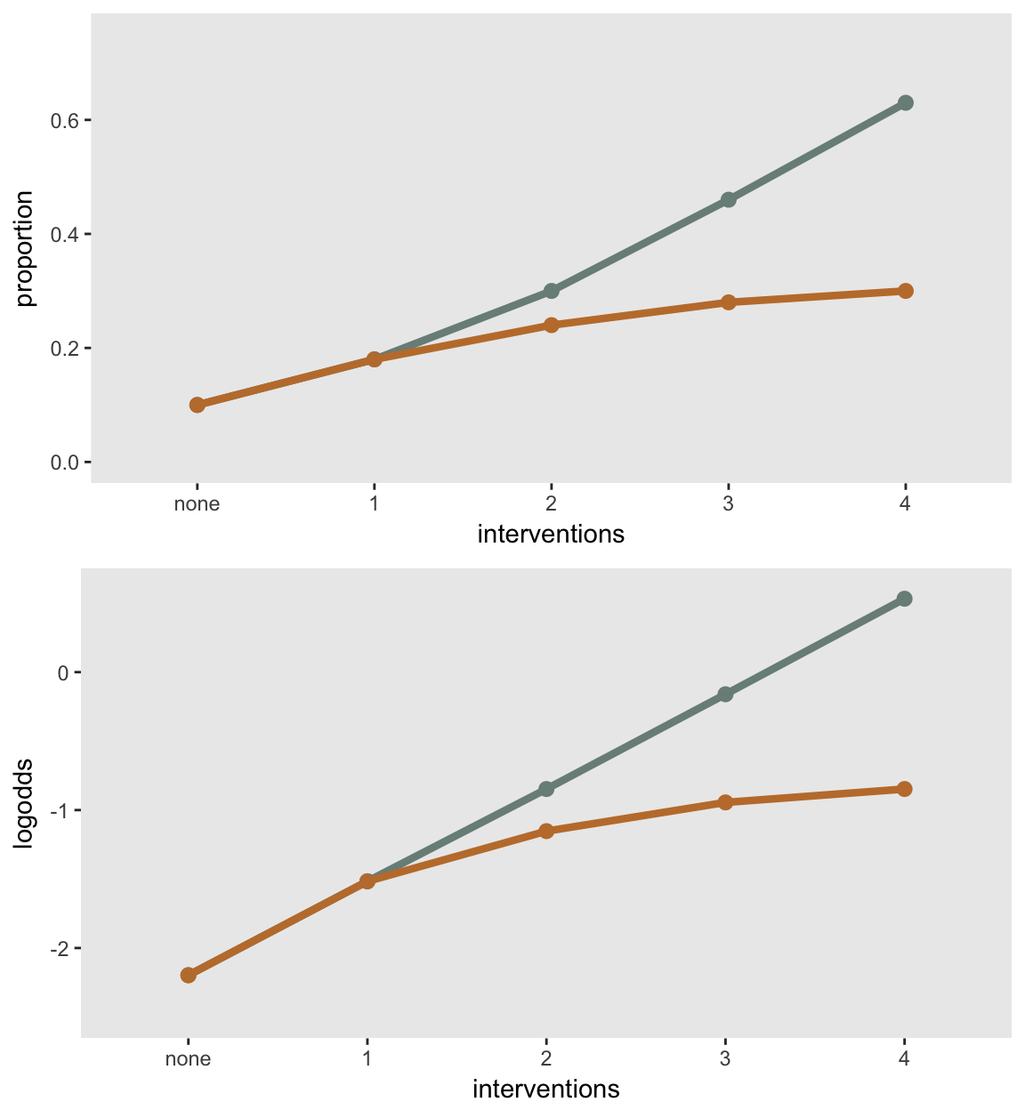
Again, we have two scenarios - one with interaction and one without. When I talk about an additive (non-interaction) model in this context, the additivity is on the log-odds scale. This becomes apparent when looking at a plot.
I want to reiterate here that we have interaction when there are limits to how much marginal effect an additional intervention can have conditional on the presence of other interventions. In a recent project (one that motivated this pair of blog entries), we started with the assumption that a single intervention would have a 5 percentage point effect on the outcome (which was smoking cessation), but a combination of all four interventions might only get a 10 percentage point reduction. This cap generates severe interaction which dramatically affected sample size requirements, as we see below (using even less restrictive interaction assumptions).
No interaction:
##                            condition formula variance   dist     link
## 1: (fac1 + fac2 + fac3 + fac4) == -4    0.10       NA binary identity
## 2: (fac1 + fac2 + fac3 + fac4) == -2    0.18       NA binary identity
## 3: (fac1 + fac2 + fac3 + fac4) ==  0    0.30       NA binary identity
## 4: (fac1 + fac2 + fac3 + fac4) ==  2    0.46       NA binary identity
## 5: (fac1 + fac2 + fac3 + fac4) ==  4    0.63       NA binary identity
Interaction:
##                            condition formula variance   dist     link
## 1: (fac1 + fac2 + fac3 + fac4) == -4    0.10       NA binary identity
## 2: (fac1 + fac2 + fac3 + fac4) == -2    0.18       NA binary identity
## 3: (fac1 + fac2 + fac3 + fac4) ==  0    0.24       NA binary identity
## 4: (fac1 + fac2 + fac3 + fac4) ==  2    0.28       NA binary identity
## 5: (fac1 + fac2 + fac3 + fac4) ==  4    0.30       NA binary identity
The plot highlights that additivity is on the log-odds scale only:

The sample size requirement for a treatment effect of 8 percentage points for a single intervention compared to control is about 640 total participants:
power.prop.test(power = 0.90, p1 = .10, p2 = .18, sig.level = 0.10)##
## Two-sample comparison of proportions power calculation
##
## n = 320.3361
## p1 = 0.1
## p2 = 0.18
## sig.level = 0.1
## power = 0.9
## alternative = two.sided
##
## NOTE: n is number in *each* groupSimulation shows that the multi-factorial experiment requires only 500 participants, a pretty surprising reduction:
dt <- genMultiFac(31, nFactors = 4, coding = "effect",
                  colNames = paste0("fac", c(1:4)))

res <- iterFunc(bNoX, dt, binary = TRUE)

apply(res$p[, .(fac1, fac2, fac3, fac4)] < 0.10, 2, mean)
## fac1 fac2 fac3 fac4
## 0.889 0.910 0.916 0.901But, if there is a cap to how much we can effect the outcome (i.e. there is underlying interaction), estimated power is considerably reduced:
dt <- genMultiFac(31, nFactors = 4, coding = "effect",
                  colNames = paste0("fac", c(1:4)))

res <- iterFunc(bX, dt, binary = TRUE)

apply(res$p[, .(fac1, fac2, fac3, fac4)] < 0.10, 2, mean)
## fac1 fac2 fac3 fac4
## 0.398 0.409 0.405 0.392We need to increase the sample size to about just to explore the main effects:
dt <- genMultiFac(125, nFactors = 4, coding = "effect",
                  colNames = paste0("fac", c(1:4)))

res <- iterFunc(bX, dt, binary = TRUE)

apply(res$p[, .(fac1, fac2, fac3, fac4)] < 0.10, 2, mean)
## fac1 fac2 fac3 fac4
## 0.910 0.890 0.895 0.887I think the biggest take away from all of this is that multi-factorial experiments are a super interesting option when exploring possible interventions or combinations of interventions, particularly when the outcome is continuous. However, this approach may not be as feasible when the outcome is binary, as sample size requirements may quickly become prohibitive, given the number of factors, sample sizes, and extent of interaction.