simstudy update - stepped-wedge design treatment assignment

Data definition

Stepped-wedge designs are a special class of cluster randomized trial where each cluster is observed in both treatment arms (as opposed to the classic parallel design where only some of the clusters receive the treatment). This is a special case of a cross-over design, where the cross-over is only in one direction: control (or pre-intervention) to intervention.

In this example, the data generating process looks like this:

\[Y_{ict} = \beta_0 + b_c + \beta_1 * t + \beta_2*X_{ct} + e_{ict}\]

where \(Y_{ict}\) is the outcome for individual \(i\) in cluster \(c\) in time period \(t\), \(b_c\) is a cluster-specific effect, \(X_{ct}\) is the intervention indicator that has a value 1 during periods where the cluster is under the intervention, and \(e_{ict}\) is the individual-level effect. Both \(b_c\) and \(e_{ict}\) are normally distributed with mean 0 and variances \(\sigma^2_{b}\) and \(\sigma^2_{e}\), respectively. \(\beta_1\) is the time trend, and \(\beta_2\) is the intervention effect.

We need to define the cluster-level variables (i.e. the cluster effect and the cluster size) as well as the individual specific outcome. In this case each cluster will have 15 individuals per period, and \(\sigma^2_b = 0.20\). In addition, \(\sigma^2_e = 1.75\).

library(simstudy)
library(ggplot2)

defc <- defData(varname = "ceffect", formula = 0, variance = 0.20, 
                dist = "normal", id = "cluster")
defc <- defData(defc, "m", formula = 15, dist = "nonrandom")

defa <- defDataAdd(varname = "Y", 
                   formula = "0 + ceffect + 0.1*period + trt*1.5", 
                   variance = 1.75, dist = "normal")

In this case, there will be 30 clusters and 24 time periods. With 15 individuals per cluster per period, there will be 360 observations for each cluster, and 10,800 in total. (There is no reason the cluster sizes need to be deterministic, but I just did that to simplify things a bit.)

Cluster-level intervention assignment is done after generating the cluster-level and time-period data. The call to trtStepWedge includes 3 key arguments that specify the number of waves, the length of each wave, and the period during which the first clusters begin the intervention.

nWaves indicates how many clusters share the same starting period for the intervention. In this case, we have 5 waves, with 6 clusters each. startPer is the first period of the first wave. The earliest starting period is 0, the first period. Here, the first wave starts the intervention during period 4. lenWaves indicates the length between starting points for each wave. Here, a length of 4 means that the starting points will be 4, 8, 12, 16, and 20.

Once the treatment assignments are made, the individual records are created and the outcome data are generated in the last step.

set.seed(608477)

dc <- genData(30, defc)
dp <- addPeriods(dc, 24, "cluster", timevarName = "t")
dp <- trtStepWedge(dp, "cluster", nWaves = 5, lenWaves = 4, 
          startPer = 4, grpName = "trt")

dd <- genCluster(dp, cLevelVar = "timeID", "m", "id")
dd <- addColumns(defa, dd)

dd

##        cluster period ceffect  m timeID startTrt trt    id     Y
##     1:       1      0   0.628 15      1        4   0     1  1.52
##     2:       1      0   0.628 15      1        4   0     2  0.99
##     3:       1      0   0.628 15      1        4   0     3 -0.12
##     4:       1      0   0.628 15      1        4   0     4  2.09
##     5:       1      0   0.628 15      1        4   0     5 -2.34
##    ---                                                          
## 10796:      30     23  -0.098 15    720       20   1 10796  1.92
## 10797:      30     23  -0.098 15    720       20   1 10797  5.92
## 10798:      30     23  -0.098 15    720       20   1 10798  4.12
## 10799:      30     23  -0.098 15    720       20   1 10799  4.57
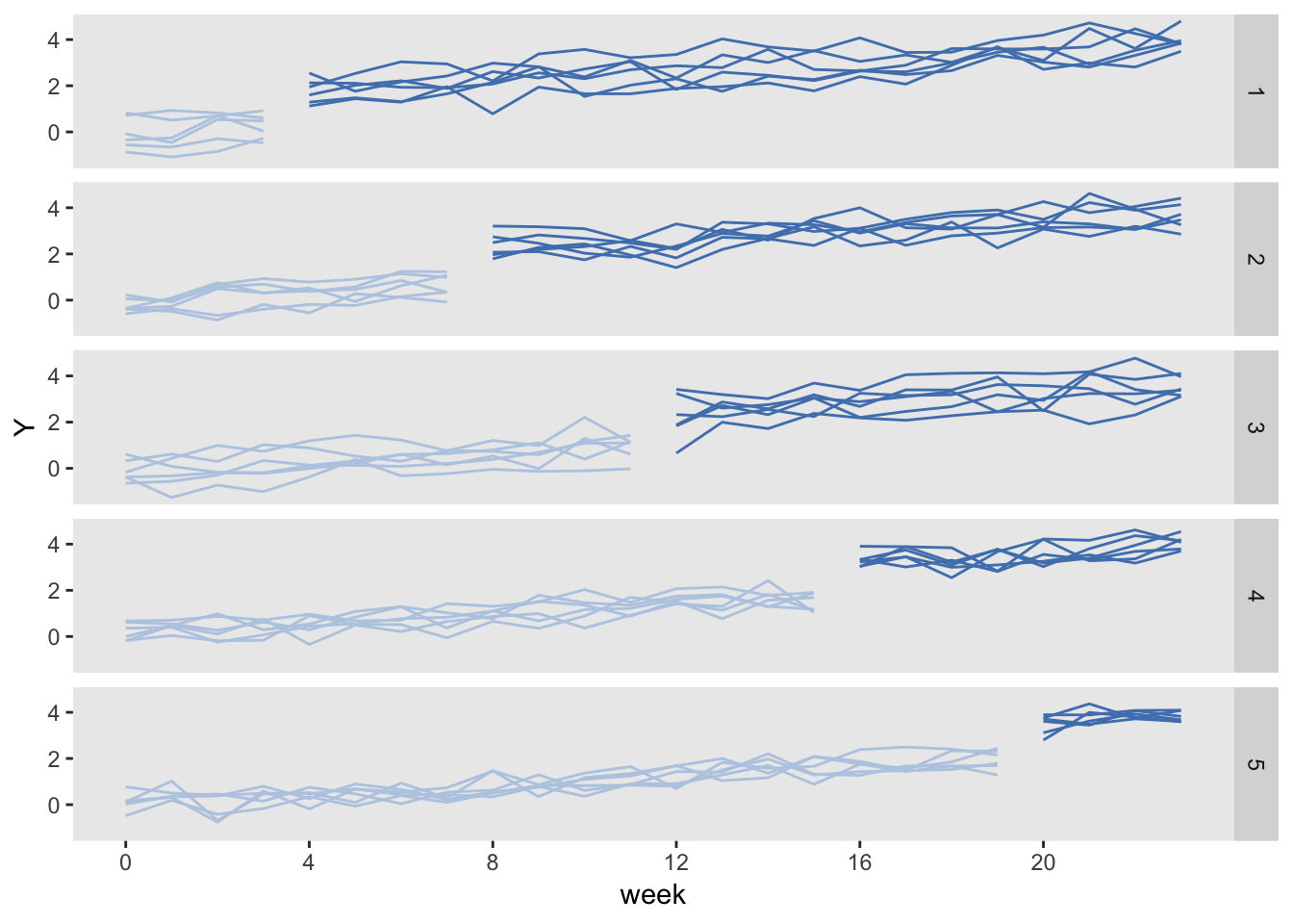
## 10800:      30     23  -0.098 15    720       20   1 10800  3.66

It is easiest to understand the stepped-wedge design by looking at it. Here, we average the outcomes by each cluster for each period and plot the results.

dSum <- dd[, .(Y = mean(Y)), keyby = .(cluster, period, trt, startTrt)]

ggplot(data = dSum, 
    aes(x = period, y = Y, group = interaction(cluster, trt))) +
  geom_line(aes(color = factor(trt))) +
  facet_grid(factor(startTrt, labels = c(1 : 5)) ~ .) +
  scale_x_continuous(breaks = seq(0, 23, by = 4), name = "week") +
  scale_color_manual(values = c("#b8cce4", "#4e81ba")) +
  theme(panel.grid = element_blank(),
        legend.position = "none") 

Key elements of the data generation process are readily appreciated by looking at the graph: (1) the cluster-specific effects, reflected in the variable starting points at period 0, (2) the general upward time trend, and (3), the stepped-wedge intervention scheme.

Since trtStepWedge is a new function, it is still a work in progress. Feel free to get in touch to give me feedback on any enhancements that folks might find useful.