I am collaborating with a number of folks who think a lot about palliative or supportive care for people who are facing end-stage disease, such as advanced dementia, cancer, COPD, or congestive heart failure. A major concern for this population (which really includes just about everyone at some point) is the quality of life at the end of life and what kind of experiences, including interactions with the health care system, they have (and don’t have) before death.
A key challenge for researchers is figuring out how to analyze events that occur just before death. For example, it is not unusual to consider hospitalization in the week or month before death as a poor outcome. For example, here is a paper in the Journal of Palliative Care Medicine that describes an association of homecare nursing and reduced hospitalizations in the week before death. While there is no denying the strength of the association, it is less clear how much of that association is causal.
In particular, there is the possibility of selection bias that may be result when considering only patients who have died. In this post, I want to describe the concept of selection bias and simulate data that mimics the process of end-stage disease in order to explore how these issues might play out when we are actually evaluating the causal effect of an exposure or randomized intervention.
Selection bias
Selection bias is used to refer to different concepts by different researchers (see this article by Haneuse or this one by Hernán et al for really nice discussions of these issues). The terminology doesn’t matter as much as understanding the underlying data generating processes that distinguish the different ideas.
The key issue is to understand what is being selected. In one case, the exposure or intervention is the focus. And in the second case, it is how the patients or subjects are selected into the study more generally that induces the bias. The first selection process is typically referred to by epidemiologists as confounding bias (though it is also called treatment-selection bias), while the second is actually selection bias.
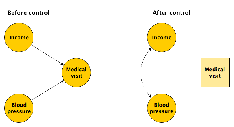
When I’ve written about these issues before (for example, see here), I’ve described how DAGs can be useful to illuminate the potential biases. Below, I have drawn a diagram to represent a simple case of selection bias. Say we are interested in measuring the causal relationship between income and blood pressure in some population in which the two are actually not causally related. If people with higher income are more likely to visit a doctor, and if people with higher blood pressure are also more likely to visit a doctor, the underlying causal relationship might be well represented by the DAG on the left in the figure below.

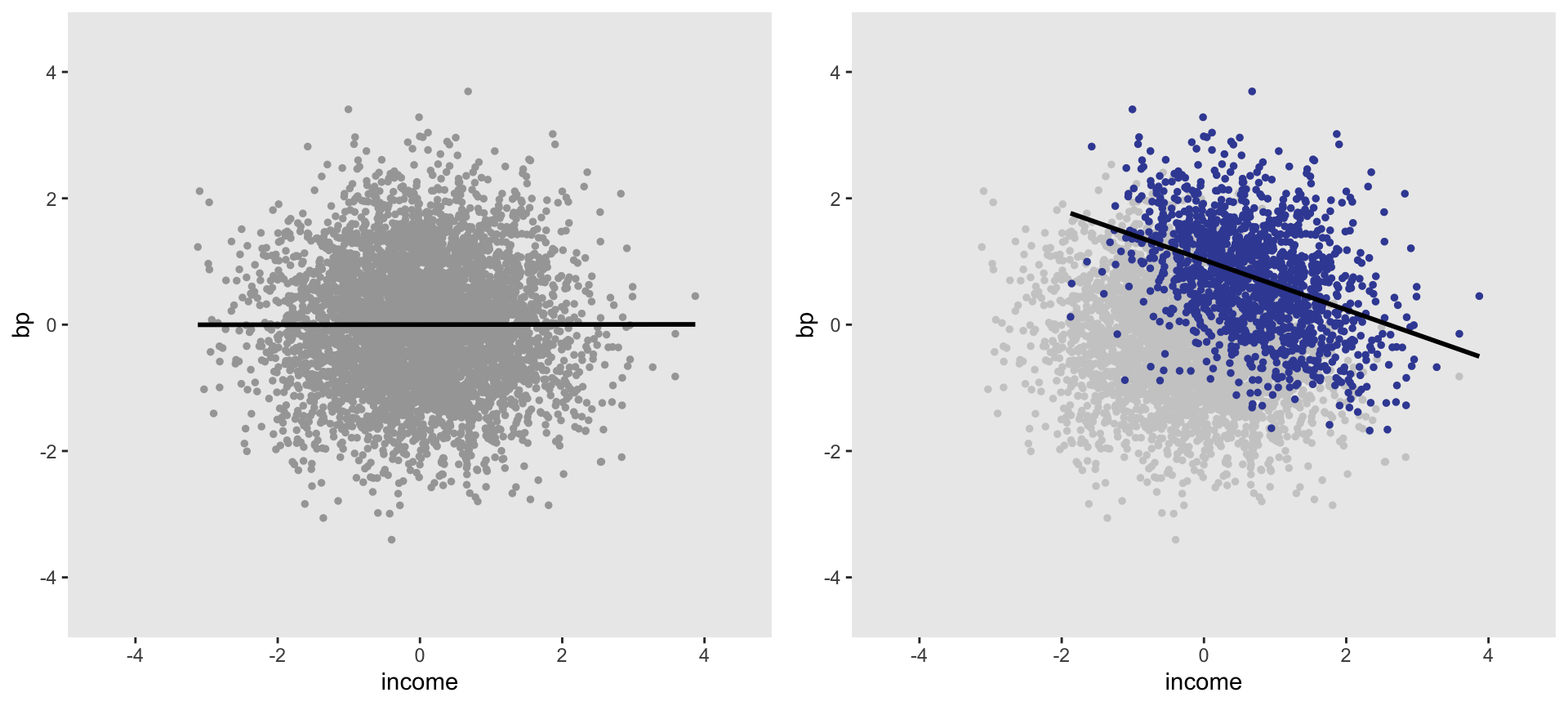
Let’s say we recruit participants for our study right outside of a medical facility. Choosing this location (as opposed to, say, a shopping mall where the causal model on the left would not be relevant), we are inducing a relationship between income and blood pressure. This can be seen in the DAG on the right, where we have effectively “controlled” for medical facility access in our selection process. The induced statistical relationship can be described in this way: if someone is at the medical center and they have relatively low income, they are more likely to have relatively high blood pressure. Conversely, if someone is there and they have relatively low blood pressure, they are more likely to have relatively high income. Based on this logic, we would expect to see a negative relationship between income and blood pressure in our study sample drawn from patients visiting a medical facility.
To explore by simulation, we can generate a large population of individuals with uncorrelated income and blood pressure. Selection will be a function of both:
n = 5000
set.seed(748347)

income <- rnorm(n);
bp <- rnorm(n)

logitSelect <- -2 + 2*income + 2*bp
pSelect <- 1/(1+exp(-logitSelect))
select <- rbinom(n, 1, pSelect)

dPop <- data.table(income, bp, select)
dSample <- dPop[select == 1]
The plot on the left below is the overall population of 5000; there is no obvious relationship between the income and blood pressure. The group that was recruited at the medical facility and enrolled in the study (a subset of the original population) is shown in purple in the plot on the right. In this subset, there does indeed appear to be a relationship between the two characteristics. An estimate of the association, which we know is zero, based on the sample would be biased; that bias is due to how we selected participants into the study.

Hospitalization before death
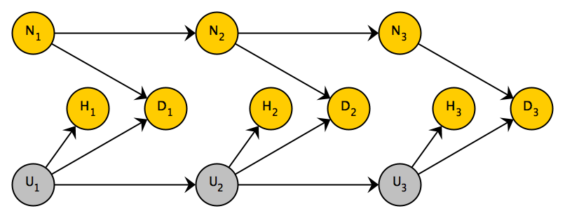
In the next simulation, let’s consider a somewhat more complex process, though with the same underlying structure and similar bias as the simpler case above. The next DAG (below) shows three different time periods. In this case there is an indicator of homecare by a nurse , , and . (In this particular example, an individual has home nursing care in all three periods or they don’t have any home nursing care in any period. This is not a requirement.) In each period, each patient has an underlying time-dependent health status, ranging from (healthiest) to (sickest). In this simulated study, the underlying health status , , and are considered latent (i.e. unmeasured). The progression of health status is governed by a Markov process that is independent of any kind of treatment. (See here and here for a more detailed description of how this is done using simstudy.)
The probability of hospitalization is a solely a function of the underlying health status, and nothing else. (I could make hospitalization a function of palliative care as well, but this just simplifies matters. In both cases the estimates will be biased - you can try for yourself.)
Death is a function of underlying health status and palliative care. While it does not seem to be the case in practice, I am assuming that less aggressive care results in shorter survival times. And the sicker the patient is in a particular period, the greater risk of dying in that period. (There should be lines between death in various periods and all subsequent measures, but I have eliminated them for clarity sake.)

The code to generate the data starts with the definitions: first, I define an initial health state that can range from 1 to 3 and the transition matrix for the Markov process. Next, I define the hospitalization and death outcomes:
bDef <- defData(varname = "S0", formula = "0.4;0.4;0.2",
                     dist = "categorical")

P <- t(matrix(c( 0.7, 0.2, 0.1, 0.0,
                 0.0, 0.4, 0.4, 0.2,
                 0.0, 0.0, 0.6, 0.4,
                 0.0, 0.0, 0.0, 1.0),
              nrow = 4))

pDef <- defDataAdd(varname = "hospital", formula = "-2 + u",
                   dist = "binary", link = "logit")
pDef <- defDataAdd(pDef, varname = "death",
                   formula = "-2 + u + homenurse * 1.5",
                   dist = "binary", link = "logit")
The data generation process randomizes individuals to nursing home care (or care as usual) in the first period, and creates all of the health status measures and outcomes. The last step removes any data for an individual that was generated after they died. (The function trimData is new and only available in simstudy 0.1.15, which is available on CRAN - as of 10/21/2019)
set.seed(272872)

dd <- genData(10000, bDef)
dd <- trtAssign(dd, grpName = "homenurse")

dp <- addMarkov(dd, transMat = P,
                chainLen = 4, id = "id",
                pername = "seq", start0lab = "S0",
                varname = "u")

dp <- addColumns(pDef, dp)
dp <- trimData(dp, seqvar = "seq", eventvar = "death")
A short follow-up period
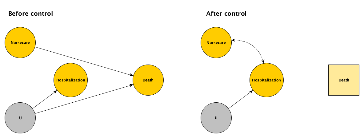
If we have a relatively short follow up period in our randomized trial of supportive care at home (nursecare), only a portion of the sample will die; as result, we can only compare the hospitalization before death for a subset of the sample. By selecting on death, we will induce a relationship between the intervention and the outcome where none truly exists. Inspecting the DAGs below, it is apparent that this is a classic case of selection bias. Since we cannot control for the unmeasured health status , hospitalization and death are associated. And, since treatment and death are causally related, by selecting on death we are in the same situation as we were in the first example.

d1 <- dp[seq == 1]If we consider only those who died in the first period, we will be including 61% of the sample:
d1[, mean(death)]## [1] 0.6109To get a sense of the bias, I am considering three models. The first model estimates the effect of the intervention on hospitalization for only those who died in the first period; we expect that this will have a negative bias. In the second model, we use the same subset of patients who died, but adjust for underlying health status; the hospitalization coefficient should be close to zero. Finally, we estimate a model for everyone in period 1, regardless of whether they died. again, we expect the effect size to be close to 0.
fit1 <- glm(hospital ~ homenurse, data=d1[death==1],
            family = "binomial")
fit2 <- glm(hospital ~ homenurse + u, data=d1[death==1],
            family = "binomial")
fit3 <- glm(hospital ~ homenurse, data=d1,
            family = "binomial")

library(stargazer)

stargazer(fit1, fit2, fit3, type = "text",
          column.labels = c("died", "died - adjusted", "all"),
          omit.stat = "all", omit.table.layout = "-asn")
##
## =============================================
## Dependent variable:
## -----------------------------------
## hospital
## died died - adjusted all
## (1) (2) (3)
## homenurse -0.222*** -0.061 -0.049
## (0.053) (0.057) (0.040)
##
## u 1.017***
## (0.039)
##
## Constant 0.108** -2.005*** -0.149***
## (0.042) (0.092) (0.028)
##
## =============================================While these are estimates from a single data set (I should really do more extensive experiment based on many different data sets), the estimates do seem to support our expectations. Indeed, if we cannot measure the underlying health status, the estimate of the intervention effect on hospitalization prior to death is biased; we would conclude that supportive care reduces the probability of hospitalization before death when we know (based on the data generation process used here) that it does not.
Extended follow-up
We might think that if we could follow everyone up until death (and hence not select on death), the bias would be eliminated. However, this not the case. The treatment effect is essentially an average of the effect over all time periods, and we know that for each time period, the effect estimate is biased due to selection. And averaging across biased estimates yields a biased estimate.
This issue is closely related to a general issue for causal survival analysis. It has been pointed out that it is not possible to estimate a causal treatment effect using hazard rates, as we do when we use Cox proportional hazard models. This is true even if treatment has been randomized and the two treatment arms are initially balanced with respect to underlying health status. The challenge is that after the first set of deaths, the treatment groups will no longer be balanced with respect to health status; some people survived because of the intervention, others because they were generally healthier. At each point in the survival analysis, the model for risk of death is conditioning (i.e. selecting on) those who did not die. So, there is built in selection bias in the modelling. If you are interested in reading more about these issues, I recommend taking a look at these papers by Hernán and Aalen et al..
Now, back to the simulation. In this case, we analyze everyone who has died within 4 periods, which is about 97% of the initial sample, virtually everyone.
dDied <- dp[death == 1]
nrow(dDied)/nrow(d1)
## [1] 0.9658The effect estimate based on this data set is only unbiased when we are able to control for underlying health status. Otherwise, extending follow-up does not help remove any bias.
fit4 <- glm(hospital ~ homenurse, data=dDied, family = "binomial")
fit5 <- glm(hospital ~ homenurse + u, data=dDied, family = "binomial")

stargazer(fit4, fit5, type = "text",
          omit.stat = "all", omit.table.layout = "-asn")
##
## ==============================
## Dependent variable:
## --------------------
## hospital
## (1) (2)
## homenurse -0.383*** -0.048
## (0.041) (0.045)
##
## u 1.020***
## (0.028)
##
## Constant 0.296*** -2.028***
## (0.030) (0.070)
##
## ==============================In the future, I hope to explore alternative ways to analyze these types of questions. In the case of survival analysis, models that do not condition on death have been proposed to get at causal estimates. This may not be possible when the outcome of interest (health care before death) is defined by conditioning on death. We may actually need to frame the question slightly differently to be able to get an unbiased estimate.
References:
Seow, H., Sutradhar, R., McGrail, K., Fassbender, K., Pataky, R., Lawson, B., Sussman, J., Burge, F. and Barbera, L., 2016. End-of-life cancer care: temporal association between homecare nursing and hospitalizations. Journal of palliative medicine, 19(3), pp.263-270.
Haneuse, S., 2016. Distinguishing selection bias and confounding bias in comparative effectiveness research. Medical care, 54(4), p.e23.
Hernán, M.A., Hernández-Díaz, S. and Robins, J.M., 2004. A structural approach to selection bias. Epidemiology, 15(5), pp.615-625.
Hernán, M.A., 2010. The hazards of hazard ratios. Epidemiology, 21(1), p.13.
Aalen, O.O., Cook, R.J. and Røysland, K., 2015. Does Cox analysis of a randomized survival study yield a causal treatment effect?. Lifetime data analysis, 21(4), pp.579-593.
Support:
This research is supported by the National Institutes of Health National Institute on Aging R33AG061904. The views expressed are those of the author and do not necessarily represent the official position of the funding organizations.