It’s always nice to be able to speed things up a bit. My first blog post ever described an approach using Rcpp to make huge improvements in a particularly intensive computational process. Here, I want to show how simple it is to speed things up by using the R package parallel and its function mclapply. I’ve been using this function more and more, so I want to explicitly demonstrate it in case any one is wondering.
I’m using a very simple power calculation as the motivating example here, but parallel processing can be useful in any problem where multiple replications are required. Monte Carlo simulation for experimentation and bootstrapping for variance estimation are other cases where computation times can grow long particularly fast.
A simple, two-sample experiment
In this example, we are interested in estimating the probability of an experiment to show some sort of treatment effect given that there actually is an effect. In this example, I am comparing two group means with an unknown but true difference of 2.7; the standard deviation within each group is 5.0. Furthermore, we know we will be limited to a sample size of 100.
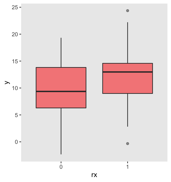
Here is the straightforward data generation process: (1) create 100 individual records, (2) assign 50 to treatment (rx) and 50 to control, and (3) generate an outcome for each individual, with and , both with standard deviation .
set.seed(2827129)

defA <- defDataAdd(varname = "y", formula ="10 + rx*2.7", variance = 25)

DT <- genData(100)
DT <- trtAssign(DT, grpName = "rx")
DX <- addColumns(defA, DT)

ggplot(data = DX, aes(factor(rx), y)) +
  geom_boxplot(fill = "red", alpha = .5) +
  xlab("rx") +
  theme(panel.grid = element_blank())
A simple linear regression model can be used to compare the group means for this particular data set. In this case, since , we would conclude that the treatment effect is indeed different from . However, in other samples, this will not necessarily be the case.
rndTidy(lm(y ~ rx, data = DX))## term estimate std.error statistic p.value
## 1: (Intercept) 9.8 0.72 13.7 0.00
## 2: rx 2.2 1.01 2.2 0.03The for loop
The single sample above yielded a . The question is, would this be a rare occurrence based on a collection of related experiments. That is, if we repeated the experiment over and over again, what proportion of the time would ? To find this out, we can repeatedly draw from the same distributions and for each draw we can estimate the p-value. (In this simple power analysis, we would normally use an analytic solution (i.e., an equation), because that is obviously much faster; but, the analytic solution is not always so straightforward or even available.)
To facilitate this replication process, it is often easier to create a function that both generates the data and provides the estimate that is needed (in this case, the p-value). This is the purposed of function genAndEst:
genAndEst <- function(def, dx) {

  DX <- addColumns(def, dx)
  coef(summary(lm(y ~ rx, data = DX)))["rx", "Pr(>|t|)"]

}
Just to show that this function does indeed provide the same p-value as before, we can call based on the same seed.
set.seed(2827129)

DT <- genData(100)
DT <- trtAssign(DT, grpName = "rx")

(pvalue <- genAndEst(defA, DT))
## [1] 0.029OK - now we are ready to estimate, using 2500 replications. Each time, we store the results in a vector called pvals. After the replications have been completed, we calculate the proportion of replications where the p-value was indeed below the threshold.
forPower <- function(def, dx, reps) {

  pvals <- vector("numeric", reps)

  for (i in 1:reps) {
    pvals[i] <- genAndEst(def, dx)
  }

  mean(pvals < 0.05)
}

forPower(defA, DT, reps = 2500)
## [1] 0.77The estimated power is 0.77. That is, given the underlying data generating process, we can expect to find a significant result of the times we conduct the experiment.
As an aside, here is the R function power.t.test, which uses the analytic (formulaic) approach:
power.t.test(50, 2.7, 5)##
## Two-sample t test power calculation
##
## n = 50
## delta = 2.7
## sd = 5
## sig.level = 0.05
## power = 0.76
## alternative = two.sided
##
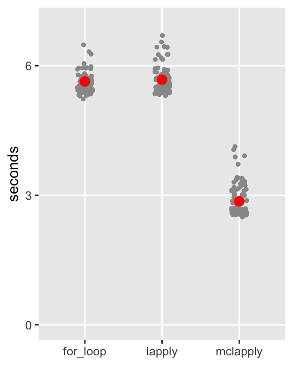
## NOTE: n is number in *each* groupReading along here, you can’t tell how much time the for loop took on my MacBook Pro. It was not exactly zippy, maybe 5 seconds or so. (The result from power.t.test was instantaneous.)
lapply
The R function lapply offers a second approach that might be simpler to code, but maybe less intuitive to understand. The whole replication process can be coded with a single call to lapply. This call also references the genAndEst function.
In this application of lapply, the argument is really a dummy argument, as the function call in argument essentially ignores the argument . lapply executes the function for each element of the vector ; in this case, the function will be executed times. That is, we get replications of the function genAndEst, just as we did with the for loop.
lappPower <- function(def, dx, reps = 1000) {

  plist <- lapply(X = 1:reps, FUN = function(x) genAndEst(def, dx))
  mean(unlist(plist) < 0.05)

}

lappPower(defA, DT, 2500)
## [1] 0.75The power estimate is quite close to the initial for loop replication and the analytic solution. However, in this case, it did not appear to provide any time savings, taking about 5 seconds as well.
mclapply
The final approach here is the mclapply function - or multi-core lapply. The syntax is almost identical to lapply, but the speed is not. It seems like it took about 2 or 3 seconds to do 2500 replications.
library(parallel)

mclPower <- function(def, dx, reps) {

  plist <- mclapply(1:reps, function(x) genAndEst(def, dx), mc.cores = 4)
  mean(unlist(plist) < 0.05)

}

mclPower(defA, DT, 2500)
## [1] 0.75Benchmarking the processing times
You’ve had to take my word about the relative processing times. Here, I use package microbenchmark to compare the three approaches (leaving out the analytic solution, because it is far, far superior in this case). This bench-marking process actually does 100 replications of each approach. And each replication involves 2500 p-value estimates. So, the benchmark takes quite a while on my laptop:
library(microbenchmark)

m1500 <- microbenchmark(for_loop = forPower(defA, DT, 1500),
               lapply = lappPower(defA, DT, 1500),
               mclapply = mclPower(defA, DT, 1500),
               times = 100L
)
The results of the benchmark are plotted here, with each of the 100 benchmark calls shown for each method, as well as the average in red. My guesstimates of the processing times were not so far off, and it looks like the parallel processing on my laptop reduces the processing times by about . In my work more generally, I have found this to be typical, and when the computation requirements are more burdensome, this reduction can really be a substantial time saver.
