This afternoon, I was looking over some simulations I plan to use in an upcoming lecture on multilevel models. I created these examples a while ago, before I started this blog. But since it was just about a year ago that I first wrote about this topic (and started the blog), I thought I’d post this now to mark the occasion.
The code below provides another way to visualize the difference between marginal and conditional logistic regression models for clustered data (see here for an earlier post that discusses in greater detail some of the key issues raised here.) The basic idea is that both models for a binary outcome are valid, but they provide estimates for different quantities.
The marginal model is estimated using a generalized estimating equation (GEE) model (here using function geeglm in package geepack). If the intervention is binary, the intervention effect (log-odds ratio) is interpreted as the average effect across all individuals regardless of the group or cluster they might belong to. (This estimate is sensitive to the relative sizes of the clusters.)
The conditional model is estimated using a random mixed effect generalized linear model (using function glmer in package lme4), and provides the log-odds ratio conditional on the cluster. (The estimate is not as sensitive to the relative sizes of the clusters since it is essentially providing a within-cluster effect.)
As the variation across clusters increases, so does the discrepancy between the conditional and marginal models. Using a generalized linear model that ignores clustering altogether will provide the correct (marginal) point estimate, but will underestimate the underlying variance (and standard errors) as long as there is between cluster variation. If there is no between cluster variation, the GLM model should be fine.
Simulation
To start, here is a function that uses simstudy to define and generate a data set of individuals that are clustered in groups. A key argument passed to this function is the across cluster variation.
library(lme4)
library(geepack)
library(broom)

genFunc <- function(nClusters, effVar) {

  # define the cluster

  def1 <- defData(varname = "clustEff", formula = 0,
                  variance = effVar, id = "cID")
  def1 <- defData(def1, varname = "nInd", formula = 40,
                  dist = "noZeroPoisson")

  # define individual level data

  def2 <- defDataAdd(varname = "Y", formula = "-2 + 2*grp + clustEff",
                     dist = "binary", link = "logit")

  # generate cluster level data

  dtC <- genData(nClusters, def1)
  dtC <- trtAssign(dtC, grpName = "grp")

  # generate individual level data

  dt <- genCluster(dtClust = dtC, cLevelVar = "cID", numIndsVar = "nInd",
                   level1ID = "id")
  dt <- addColumns(def2, dt)

  return(dt)

}
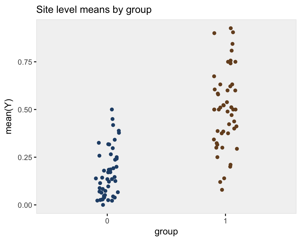
A plot of the average site level outcome from data generated with across site variance of 1 (on the log-odds scale) shows the treatment effect:
set.seed(123)
dt <- genFunc(100, 1)
dt
## cID grp clustEff nInd id Y
## 1: 1 0 -0.5604756 35 1 1
## 2: 1 0 -0.5604756 35 2 0
## 3: 1 0 -0.5604756 35 3 0
## 4: 1 0 -0.5604756 35 4 0
## 5: 1 0 -0.5604756 35 5 0
## ---
## 3968: 100 1 -1.0264209 45 3968 0
## 3969: 100 1 -1.0264209 45 3969 0
## 3970: 100 1 -1.0264209 45 3970 1
## 3971: 100 1 -1.0264209 45 3971 0
## 3972: 100 1 -1.0264209 45 3972 0dplot <- dt[, mean(Y), keyby = .(grp, cID)]
davg <- dt[, mean(Y)]
ggplot(data = dplot, aes(x=factor(grp), y = V1)) +
geom_jitter(aes(color=factor(grp)), width = .10) +
theme_ksg("grey95") +
xlab("group") +
ylab("mean(Y)") +
theme(legend.position = "none") +
ggtitle("Site level means by group") +
scale_color_manual(values = c("#264e76", "#764e26"))
Model fits
First, the conditional model estimates a log-odds ratio of 1.89, close to the actual log-odds ratio of 2.0.
glmerFit <- glmer(Y ~ grp + (1 | cID), data = dt, family="binomial")
tidy(glmerFit)
## term estimate std.error statistic p.value group
## 1 (Intercept) -1.8764913 0.1468104 -12.781729 2.074076e-37 fixed
## 2 grp 1.8936999 0.2010359 9.419711 4.523292e-21 fixed
## 3 sd_(Intercept).cID 0.9038166 NA NA NA cIDThe marginal model that takes into account clustering yields an estimate of 1.63. This model is not wrong, just estimating a different quantity:
geeFit <- geeglm(Y ~ grp, family = binomial, data = dt,
                 corstr = "exchangeable", id = dt$cID)
tidy(geeFit)
## term estimate std.error statistic p.value
## 1 (Intercept) -1.620073 0.1303681 154.42809 0
## 2 grp 1.628075 0.1740666 87.48182 0The marginal model that ignores clustering also estimates a log-odds ratio, 1.67, but the standard error estimate is much smaller than in the previous model (0.076 vs. 0.174). We could say that this model is not appropriate given the clustering of individuals:
glmFit <- glm(Y ~ grp, data = dt, family="binomial")
tidy(glmFit)
## term estimate std.error statistic p.value
## 1 (Intercept) -1.639743 0.0606130 -27.05267 3.553136e-161
## 2 grp 1.668143 0.0755165 22.08978 3.963373e-108Multiple replications
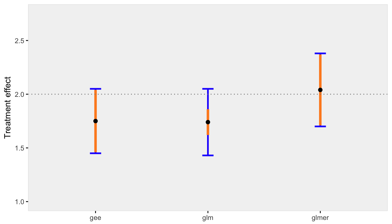
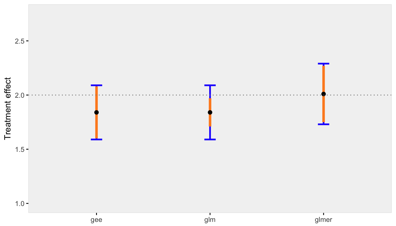
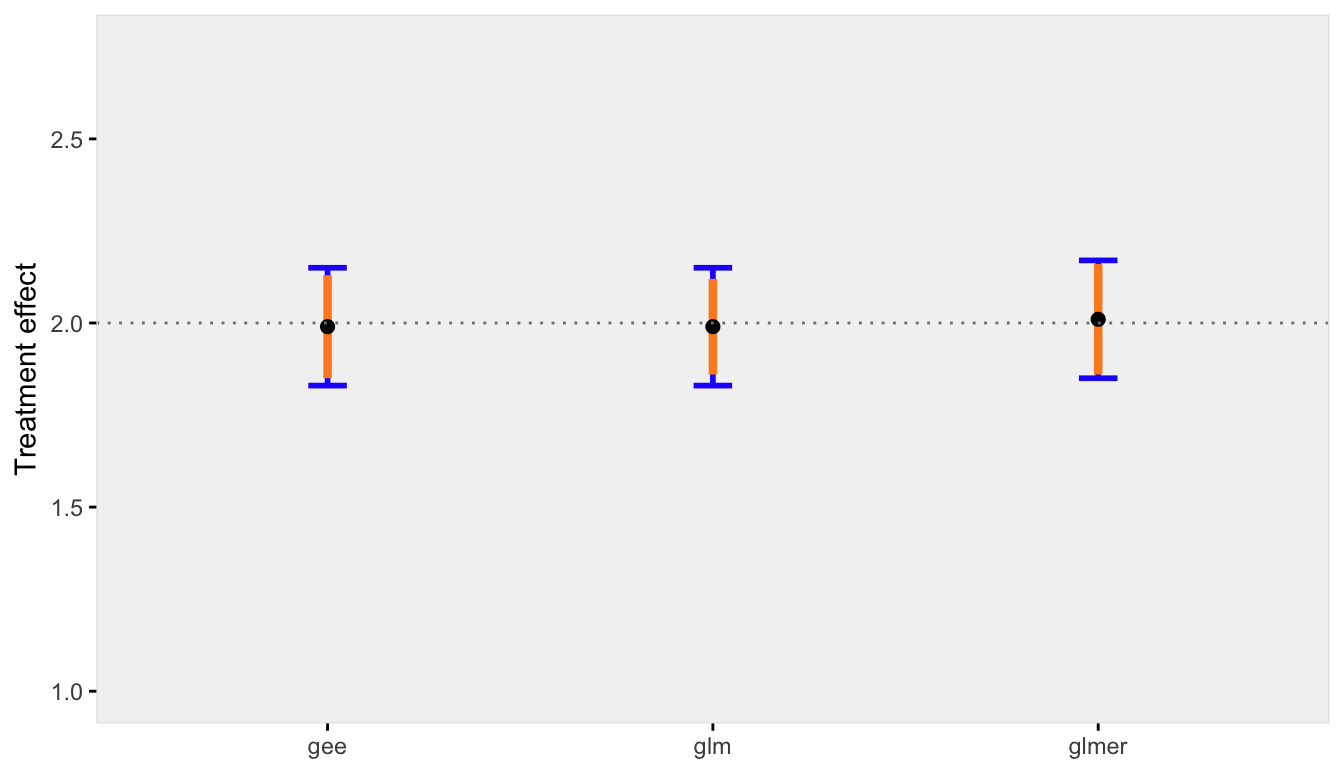
With multiple replications (in this case 100), we can see how each model performs under different across cluster variance assumptions. I have written two functions (that are shown at the end in the appendix) to generate multiple datasets and create a plot. The plot shows (1) the average point estimate across all the replications in black, (2) the true standard deviation of all the point estimates across all replications in blue, (3) the average estimate of the standard errors in orange.
In the first case, the variability across sites is highest. The discrepancy between the marginal and conditional models is relatively large, but both the GEE and mixed effects models estimate the standard errors correctly (the orange line overlaps perfectly with blue line). The generalized linear model, however, provides a biased estimate of the standard error - the orange line does not cover the blue line:
set.seed(235)

res1.00 <- iterFunc(40, 1.00, 100)
s1 <- sumFunc(res1.00)
s1$p
When the across cluster variation is reduced, the discrepancy between the marginal and conditional models is reduced, as is the bias of standard error estimate for the GLM model:
res0.50 <- iterFunc(40, 0.50, 100)
s2 <- sumFunc(res0.50)
s2$p
Finally, when there is negligible variation across sites, the conditional and marginal models are pretty much one and the same. And even the GLM model that ignores clustering is unbiased (which makes sense, since there really is no clustering):
res0.05 <- iterFunc(40, 0.05, 100)
s3 <- sumFunc(res0.05)
s3$p
Appendix
Here are the two functions that generated the the replications and created the plots shown above.
iterFunc <- function(nClusters, effVar, iters = 250) {

  results <- list()

  for (i in 1:iters) {

    dt <- genFunc(nClusters, effVar)

    glmerFit <- glmer(Y ~ grp + (1 | cID), data = dt, family="binomial")
    glmFit <- glm(Y ~ grp, data = dt, family="binomial")
    geeFit <- geeglm(Y ~ grp, family = binomial, data = dt,
                     corstr = "exchangeable", id = dt$cID)

    res <- unlist(c(coef(summary(glmerFit))[2,1:2],
                    coef(summary(glmFit))[2,1:2],
                    as.vector(coef(summary(geeFit))[2,1:2])))

    results[[i]] <- data.table(t(res))

  }

  return(rbindlist(results))

}

sumFunc <- function(dtRes, precision = 2) {

  setnames(dtRes, c("estGlmer", "sdGlmer",
                    "estGlm","sdGlm",
                    "estGEE", "sdGEE"))

  meanEst <- round(apply(dtRes[, c(1, 3, 5)], 2, mean), precision)
  estSd <- round(sqrt(apply(dtRes[, c(2, 4, 5)]^2, 2, mean)), precision)
  sdEst <- round(apply(dtRes[, c(1, 3, 5)], 2, sd), precision)

  x <- data.table(rbind(c(meanEst[1], estSd[1], sdEst[1]),
                        c(meanEst[2], estSd[2], sdEst[2]),
                        c(meanEst[3], estSd[3], sdEst[3])
  ))

  setnames(x, c("estMean","estSD","sd"))
  x[, method := c("glmer","glm","gee")]

  p <- ggplot(data = x, aes(x = method, y = estMean)) +
    geom_errorbar(aes(ymin = estMean - sd, ymax = estMean + sd),
                  width = 0.1, color = "#2329fe", size = 1) +
    geom_errorbar(aes(ymin = estMean - estSD, ymax = estMean + estSD),
                  width = 0.0, color = "#fe8b23", size = 1.5) +
    geom_point(size = 2) +
    ylim(1,2.75) +
    theme_ksg("grey95") +
    geom_hline(yintercept = 2, lty = 3, color = "grey50") +
    theme(axis.title.x = element_blank()) +
    ylab("Treatment effect")

  return(list(mean=meanEst, sd=sdEst, p=p))
}