The odds ratio always confounds: while it may be constant across different groups or clusters, the risk ratios or risk differences across those groups may vary quite substantially. This makes it really hard to interpret an effect. And then there is inconsistency between marginal and conditional odds ratios, a topic I seem to be visiting frequently, most recently last month.
My aim here is to generate a few figures that might highlight some of these issues.
Assume that there is some exposure (indicated by the use of a \(1\) or \(0\) subscript) applied across a number of different groups or clusters of people (think different regions, hospitals, schools, etc.) - indicated by some number or letter \(i\). Furthermore, assume that the total number exposed at each location is the same as the number unexposed: \(N_{i0} = N_{i1} = N = 100\).
The number of folks with exposure at a particular location \(i\) who have a poor outcome is \(n_{i1}\) and the number with a good outcome is \(N-n_{i1}\). Likewise, the corresponding measures for folks not exposed are \(n_{i0}\) and \(N-n_{i0}\). The probabilities of a poor outcome for exposed and non-exposed are \(n_{i1}/N\) and \(n_{i0}/N\). The relative risk of a poor outcome for those exposed compared to those non exposed is
\[\text{RR}_i = \frac{n_{i1}/N}{n_{i0}/N} = \frac{n_{i1}}{n_{i0}},\] the risk difference between exposed and unexposed groups is
\[ \text{RD}_i = \frac{n_{i1}}{N}-\frac{n_{i0}}{N} = \frac{n_{i1} - n_{i0}}{N},\] and the odds ratio is
\[ \text{OR}_i = \frac{[n_{i1}/N] / [(N - n_{i1})/N]}{[n_{i0}/N] / [(N - n_{i0})/N]} \] \[= \frac{n_{i1}(N-n_{i0})}{n_{i0}(N-n_{i1})}.\]
The simple conditional logistic regression model that includes a group-level random effect \(b_i\) assumes a constant odds ratio between exposed and unexposed individuals across the different clusters:
\[\text{logit} (Y_{ij}) = \beta_0 + \beta_1 E_{ij} + b_i,\] where \(E_{ij}\) is an exposure indicator for person \(j\) in group \(i\). The parameter \(\text{exp}(\beta_1)\) is an estimate of the odds ratio defined above.
The point of all of this is to illustrate that although the odds-ratio is the same across all groups/clusters (i.e., there is no \(i\) subscript in \(\beta_1\) and \(\text{OR}_i = \text{OR}\)), the risk ratios and risk differences can vary greatly across groups, particularly if the \(b\)’s vary considerably.
Constant odds ratio, different risk ratios and differences
If the odds ratio is constant and we know \(n_{i1}\), we can perform a little algebraic maneuvering on the \(\text{OR}\) formula above to find \(n_{i0}\):
\[ n_{i0} = \frac{N \times n_{i1}}{\text{OR} \times (N - n_{i1}) + n_{i1}}\]
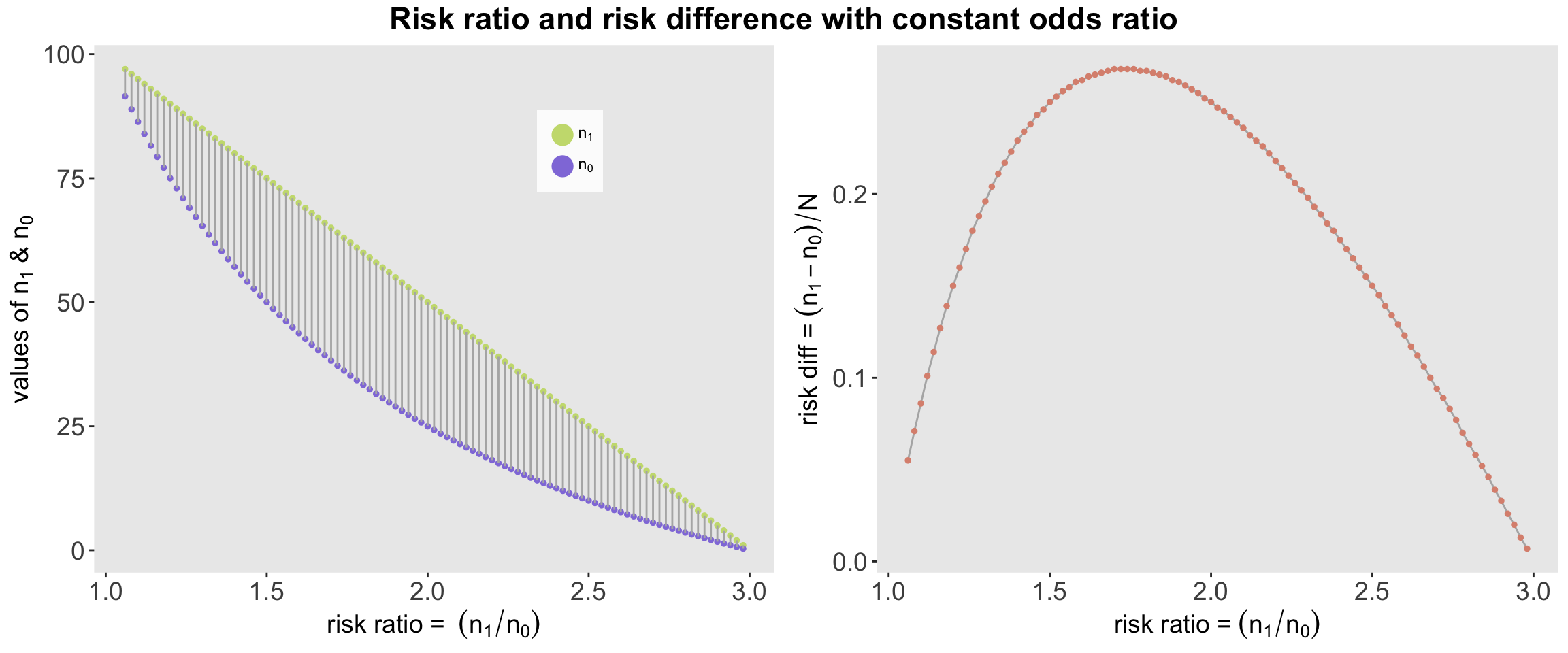
If we assume that the \(n_{i1}\)’s can range from 2 to 98 (out of 100), we can see how the risk ratios and risk differences vary considerably even though we fix the odds ratio fixed at a value of 3 (don’t pay too close attention to the fact the \(n_0\) is not an integer - this is just an illustration that makes a few violations - if I had used \(N=1000\), we could have called this rounding error):
N <- 100
trueOddsRatio <- 3

n1 <- seq(2:98)
n0 <- (N * n1)/(trueOddsRatio * (N - n1) + n1)

oddsRatio <- ((n1 / (N - n1) ) / (n0 / (N - n0) ))
riskRatio <- n1 / n0
riskDiff <- (n1 - n0) / N

dn <- data.table(n1 = as.double(n1), n0, oddsRatio,
                 riskRatio, riskDiff = round(riskDiff,3))
dn[1:6]
## n1 n0 oddsRatio riskRatio riskDiff
## 1: 1 0.3355705 3 2.98 0.007
## 2: 2 0.6756757 3 2.96 0.013
## 3: 3 1.0204082 3 2.94 0.020
## 4: 4 1.3698630 3 2.92 0.026
## 5: 5 1.7241379 3 2.90 0.033
## 6: 6 2.0833333 3 2.88 0.039With a constant odds ratio of 3, the risk ratios range from 1 to 3, and the risk differences range from almost 0 to just below 0.3. The odds ratio is not exactly informative with respect to these other two measures. The plots - two takes on the same data - tell a better story:

Another look at contrasting marginal vs conditional odds ratios
Using this same simple framework, I thought I’d see if I can illustrate the relationship between marginal and conditional odds ratios.
In this case, we have two groups/clusters where the conditional odds ratios are equivalent, yet when we combine the groups into a single entity, the combined (marginal) odds ratio is less than each of the conditional odds ratios.
In this scenario each cluster has 100 people who are exposed and 100 who are not, as before. \(a_1\) and \(a_0\) represent the number of folks with a poor outcome for the exposed and unexposed in the first cluster, respectively; \(b_1\) and \(b_0\) represent the analogous quantities in the second cluster. As before \(a_0\) and \(b_0\) are derived as a function of \(a_1\) and \(b_1\), respectively, and the constant odds ratio.
constantOR <- function(n1, N, OR) {
  return(N*n1 / (OR*(N-n1) + n1))
}


# Cluster A

a1 <- 55
a0 <- constantOR(a1, N = 100, OR = 3)
(a1*(100 - a0)) / (a0 * (100 - a1))
## [1] 3# Cluster B
b1 <- 35
b0 <- constantOR(b1, N = 100, OR = 3)
(b1*(100 - b0)) / (b0 * (100 - b1))## [1] 3# Marginal OR
tot0 <- a0 + b0
tot1 <- a1 + b1
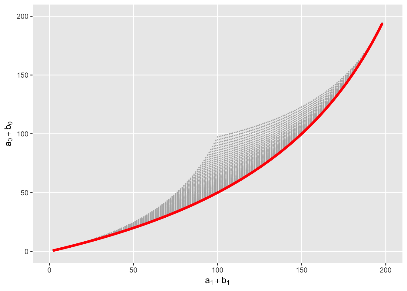
(tot1*(200 - tot0)) / (tot0 * (200 - tot1))## [1] 2.886952For this example, the marginal odds ratio is less than the conditional odds ratio. How does this contrast between the marginal and conditional odds ratio play out with a range of possible outcomes - all meeting the requirement of a constant conditional odds ratio? (Note we are talking about odds ratio larger than 1; everything is flipped if the OR is < 1.) The plot below shows possible combinations of sums \(a_1 + b_1\) and \(a_0 + b_0\), where the constant conditional odds ratio condition holds within each group. The red line shows all points where the marginal odds ratio equals the conditional odds ratio (which happens to be 3 in this case):

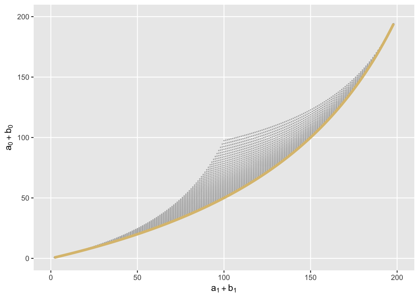
Here is the same plot, but a yellow line is drawn in all cases where \(a_1 = b_1\) (hence \(a_0 = b_0\)). This line is the directly over the earlier line where the marginal odds ratios equal 3. So, sort of proof by plotting. The marginal odds ratio appears to equal the conditional odds ratio when the proportions of each group are equal.

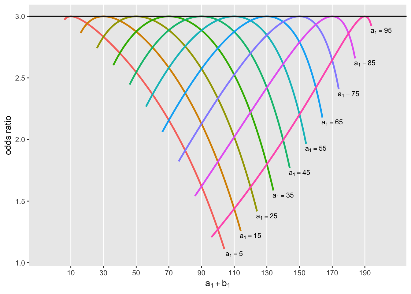
But are the marginal odds ratios not on the colored lines higher or lower than 3? To check this, look at the next figure. In this plot, the odds ratio is plotted as a function of \(a_1 + b_1\), which represents the total number of poor outcomes in the combined exposed groups. Each line represents the marginal odds ratio for a specific value of \(a_1\).

If you notice, the odds ratio reaches the constant conditional odds ratio (which is 3) only when \(a_1 + b_1 = 2a_1\), or when \(a_1 = b_1\). It appears then, when \(a_1 \ne b_1\), the marginal odds ratio lies below the conditional odds ratio. Another “proof” by figure. OK, not a proof, but colorful nonetheless.