In my previous post, I described a (relatively) simple way to simulate observational data in order to compare different methods to estimate the causal effect of some exposure or treatment on an outcome. The underlying data generating process (DGP) included a possibly unmeasured confounder and an instrumental variable. (If you haven’t already, you should probably take a quick look.)
A key point in considering causal effect estimation is that the average causal effect depends on the individuals included in the average. If we are talking about the causal effect for the population - that is, comparing the average outcome if everyone in the population received treatment against the average outcome if no one in the population received treatment - then we are interested in the average causal effect (ACE).
However, if we have an instrument, and we are talking about only the compliers (those who don’t get the treatment when not encouraged but do get it when they are encouraged) - then we will be measuring the complier average causal effect (CACE). The CACE is a comparison of the average outcome when all compliers receive the treatment with the average outcome when none of the compliers receive the treatment.
And the third causal effect I will consider here is the average causal effect for the treated (ACT). This population is defined by those who actually received the treatment (regardless of instrument or complier status). Just like the other causal effects, the ACT is a comparison of the average outcome when all those who were actually treated did get treatment (this is actually what we observe) with the average outcome if all those who were actually treated didn’t get the treatment (the counterfactual of the treated).
As we will see in short order, three different estimation methods using (almost) the same data set provide estimates for each of these three different causal estimands.
The data generating process
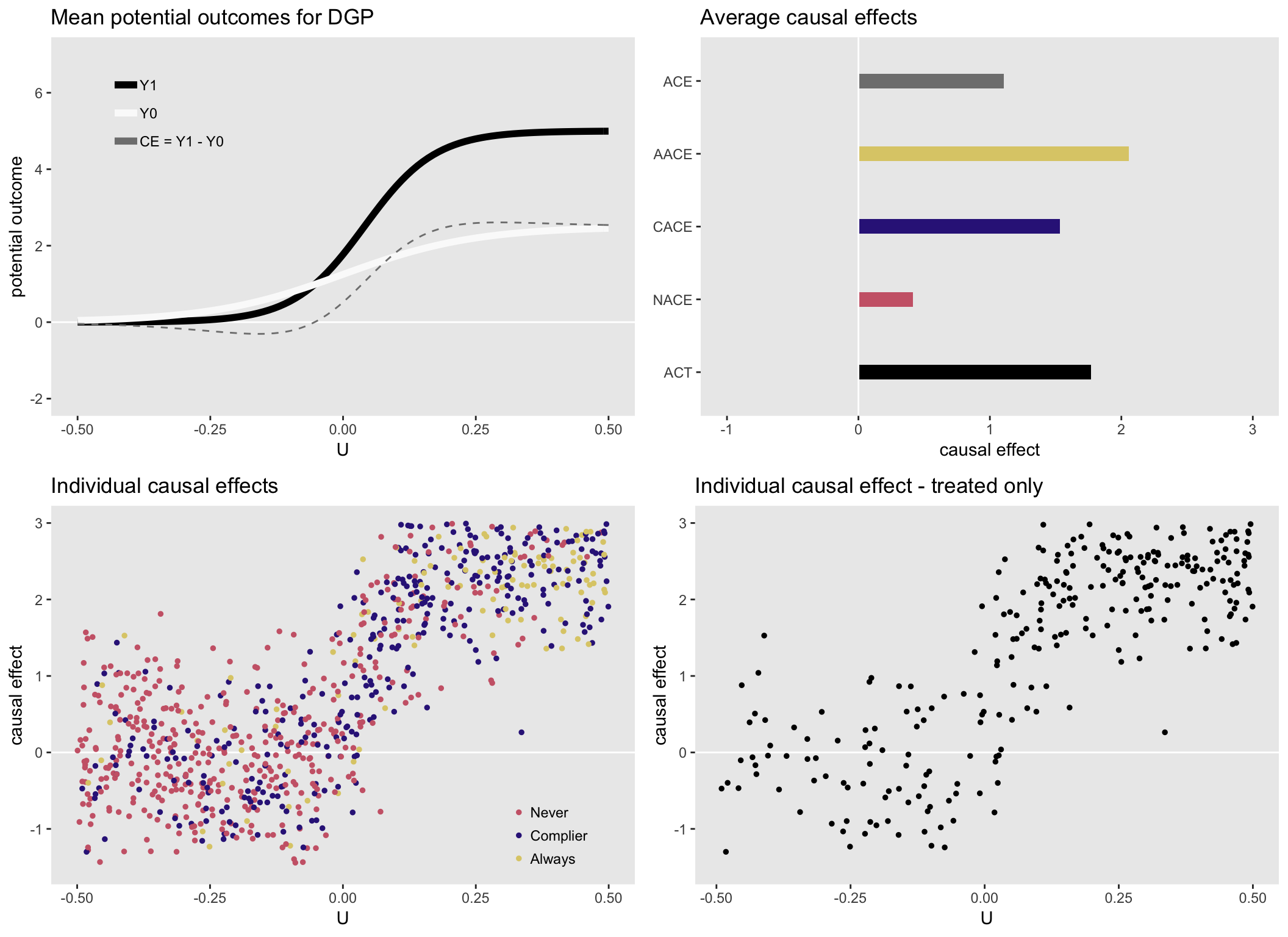
For the purposes of this illustration, I am generating data with heterogeneous causal effects that depend on an measured or unmeasured underlying health status . (I’m skipping over the details of the DGP that I laid out in part I.) Higher values of indicate a sicker patient. Those patients are more likely to have stronger effects, and are more likely to seek treatment (independent of the instrument).
Here is a set of plots that show the causal effects by health status and various distributions of the causal effects:

Instrumental variable
First up is IV estimation. The two-stage least squares regression method has been implemented in the R package ivpack. In case you didn’t check out the IV reference last time, here is an excellent tutorial that describes IV methods in great, accessible detail. The model specification requires the intervention or exposure variable (in this case ) and the instrument ().
library(ivpack)

ivmodel <- ivreg(formula = Y ~ T | A, data = DT)
broom::tidy(ivmodel)
## # A tibble: 2 x 5
## term estimate std.error statistic p.value
## <chr> <dbl> <dbl> <dbl> <dbl>
## 1 (Intercept) 1.30 0.0902 14.4 6.11e-43
## 2 T 1.52 0.219 6.92 8.08e-12The causal effect that IV methods is often called the local area treatment effect (LATE), which is just another way to talk about the CACE. Essentially, IV is estimating the causal effect for people whose behavior is modified (or would be modified) by the instrument. If we calculate the average CACE using the (unobservable) potential outcomes data for the compliers, the estimate is quite close to the IV estimate of 1.52:
DT[fS == "Complier", mean(Y1 - Y0)]## [1] 1.53Propensity score matching
If we were somehow able to measure , the underlying health status, we would be in a position to estimate the average causal effect for the treated, what I have been calling ACT, using propensity score matching. The idea here is to create a comparison group from the untreated sample that looks similar to the treated in every way except for treatment. This control is designed to be the counterfactual for the treated.
One way to do this is by matching on the propensity score - the probability of treatment. (See this article on propensity score methods for a really nice overview on the topic.)
To estimate the probability of treatment, we fit a “treatment” model, in this case a logistic generalized linear model since the treatment is binary. From this model, we can generate a predicted value for each individual. We can use software, in this case the R package Matching, to find individuals in the untreated group who share the exact or very similar propensity for treatment. Actually in this case, I will “match with replacement” so that while each treated individual will be included once, some controls might be matched with more than one treated (and those that are included repeatedly will be counted multiple times in the data).
It turns out that when we do this, the two groups will be balanced on everything that matters. In this case, the “everything”" that matters is only health status . (We actually could have matched directly on here, but I wanted to show propensity score matching, which is useful when there are many confounders that matter, and matching on them separately would be extremely difficult or impossible.)
Once we have the two groups, all we need to do is take the difference of the means of the two groups and that will give us an estimate for ACT. We could use bootstrapping methods to estimate the standard error. Below, we will use Monte Carlo simulation, so that will give us sense of the variability.
library(Matching)

# Treatment model and ps estimation

glm.fit <- glm(T ~ U, family=binomial, data=DT)
DT$ps = predict(glm.fit,type="response")

setkey(DT, T, id)

TR = DT$T
X = DT$ps

# Matching with replacement

matches <- Match(Y = NULL, Tr = TR, X = X, ties = FALSE, replace = TRUE)

# Select matches from original dataset

dt.match <- DT[c(matches$index.treated, matches$index.control)]

# ACT estimate

dt.match[T == 1, mean(Y)] - dt.match[T == 0, mean(Y)]
## [1] 1.79Once again, the matching estimate is quite close to the “true” value of the ACT calculated using the potential outcomes:
DT[T == 1, mean(Y1 - Y0)]## [1] 1.77Inverse probability weighting
This last method also uses the propensity score, but as a weight, rather than for the purposes of matching. Each individual weight is the inverse probability of receiving the treatment they actually received. (I wrote a series of posts on IPW; you can look here if you want to see a bit more.)
To implement IPW in this simple case, we just calculate the weight based on the propensity score, and use that weight in a simple linear regression model:
DT[, ipw :=  1 / ((ps * T) + ( (1 - ps) * (1 - T) ))]

lm.ipw <- lm(Y ~ T, weights = DT$ipw, data = DT)
broom::tidy(lm.ipw)
## # A tibble: 2 x 5
## term estimate std.error statistic p.value
## <chr> <dbl> <dbl> <dbl> <dbl>
## 1 (Intercept) 1.21 0.0787 15.3 1.06e-47
## 2 T 1.02 0.110 9.28 1.04e-19The IPW estimate is quite close to the estimate of the average causal effect (ACE). That is, the IPW is the marginal average:
DT[, mean(Y1 - Y0)]## [1] 1.1Randomized clinical trial
If we can make the assumption that is not the instrument but is the actual randomization and that everyone is a complier (i.e. everyone follows the randomized protocol), then the estimate we get from comparing treated with controls will also be quite close to the ACE of 1.1. So, the randomized trial in its ideal execution provides an estimate of the average causal effect for the entire sample.
randtrial <- lm(Y.r ~ A, data = DT)
broom::tidy(randtrial)
## # A tibble: 2 x 5
## term estimate std.error statistic p.value
## <chr> <dbl> <dbl> <dbl> <dbl>
## 1 (Intercept) 1.22 0.0765 15.9 5.35e-51
## 2 A 1.09 0.108 10.1 8.26e-23Intention-to-treat from RCT
Typically, however, in a randomized trial, there isn’t perfect compliance, so randomization is more like strong encouragement. Studies are typically analyzed using an intent-to-treat approach, doing the analysis as if protocol was followed correctly. This method is considered conservative (in the sense that the estimated effect is closer to 0 than true ACE is), because many of those assumed to have been treated were not actually treated, and vice versa. In this case, the estimated ITT quantity is quite a bit smaller than the estimate from a perfectly executed RCT (which is the ACE):
itt.fit <- lm(Y ~ A, data = DT)
broom::tidy(itt.fit)
## # A tibble: 2 x 5
## term estimate std.error statistic p.value
## <chr> <dbl> <dbl> <dbl> <dbl>
## 1 (Intercept) 1.50 0.0821 18.3 1.34e-64
## 2 A 0.659 0.116 5.68 1.76e- 8Per protocol analysis from RCT
Yet another approach to analyzing the data is to consider only those cases that followed protocol. So, for those randomized to treatment, we would look only at those who actually were treated. And for those randomized to control, we would only look at those who did not get treatment. It is unclear what this is actually measuring since the two groups are not comparable: the treated group includes both compliers and always-takers, whereas the control group includes both compliers and never-takers. If always-takers have larger causal effects on average and never-takers have smaller causal effects on average, the per protocol estimate will be larger than the average causal effect (ACE), and will not represent any other obvious quantity.
And with this data set, this is certainly the case:
DT[A == 1 & T == 1, mean(Y)] - DT[A == 0 & T == 0, mean(Y)] ## [1] 2.22Monte Carlo simulation
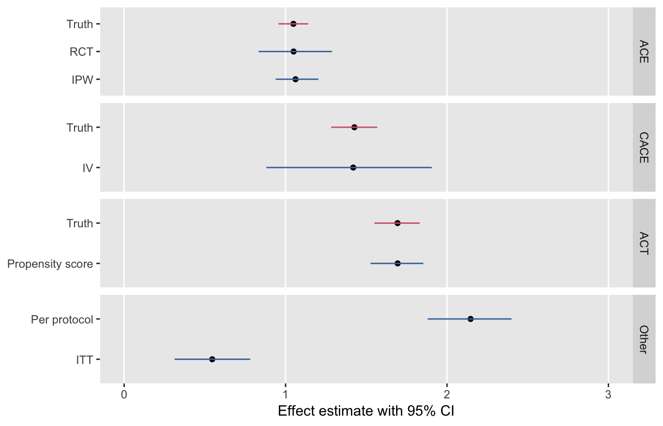
I leave you with a figure that shows the point estimates and 95% confidence intervals for each of these methods. Based on 1000 replications of the data set, this series of plots underscores the relationship of the methods to the various causal estimands.
