Correlated longitudinal data with varying time intervals

I was recently contacted to see if simstudy can create a data set of correlated outcomes that are measured over time, but at different intervals for each individual. The quick answer is there is no specific function to do this. However, if you are willing to assume an “exchangeable” correlation structure, where measurements far apart in time are just as correlated as measurements taken close together, then you could just generate individual-level random effects (intercepts and/or slopes) and pretty much call it a day. Unfortunately, the researcher had something more challenging in mind: he wanted to generate auto-regressive correlation, so that proximal measurements are more strongly correlated than distal measurements.

As is always the case with R, there are certainly multiple ways to do tackle this problem. I came up with this particular solution, which I thought I’d share. The idea is pretty simple: first, generate the time data with varying intervals, which can be done using simstudy; second, create an alternate data set of “latent” observations that include all time points, also doable with simstudy; last, merge the two in a way that gives you what you want.

Step 1: varying time intervals

The function addPeriods can create intervals of varying lengths. The function determines if the input data set includes the special fields mInterval and vInterval. If so, a time value is generated from a gamma distribution with mean mInterval and dispersion vInterval.

maxTime <- 180 # limit follow-up time to 180 days

def1 <- defData(varname = "nCount", dist = "noZeroPoisson", 
                formula = 20)
def1 <- defData(def1, varname = "mInterval", dist = "nonrandom", 
                formula = 20)
def1 <- defData(def1, varname = "vInterval", dist = "nonrandom", 
                formula = 0.4)

set.seed(20190101)
dt <- genData(1000, def1)
dtPeriod <- addPeriods(dt)
dtPeriod <- dtPeriod[time <= maxTime]

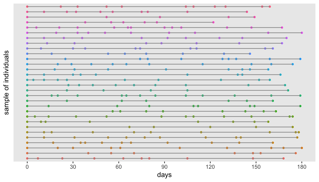
Here is a plot if time intervals for a small sample of the data set:

Step 2: generate correlated data

In this step, I am creating 181 records for each individual (from period = 0 to period = 180). In order to create correlated data, I need to specify the mean and variance for each observation; in this example, the mean is a quadratic function of time and the variance is fixed at 9. I generate the correlated data using the addCorGen function, and specify an AR-1 correlation structure with \(\rho = 0.4\),

def2 <- defDataAdd(varname = "mu", dist = "nonrandom", 
    formula = "2 + (1/500) * (time) * (180 - time)")
def2 <- defDataAdd(def2, varname = "var", dist = "nonrandom", formula = 9)

dtY <- genData(1000)
dtY <- addPeriods(dtY, nPeriod = (maxTime + 1) ) 
setnames(dtY, "period", "time")
dtY <- addColumns(def2, dtY)

dtY <- addCorGen(dtOld = dtY, idvar = "id", nvars = (maxTime + 1), 
                  rho = .4, corstr = "ar1", dist = "normal", 
                  param1 = "mu", param2 = "var", cnames = "Y")

dtY[, `:=`(timeID = NULL, var = NULL, mu = NULL)]

Here is a plot of a sample of individuals that shows the values of \(Y\) at every single time point (not just the time points generated in step 1). The \(Y\)’s are correlated within individual.

Step 3

Now we just do an inner-join, or perhaps it is a left join - hard to tell, because one data set is a subset of the other. In any case, the new data set includes all the rows from step 1 and the ones that match from step 2.

setkey(dtY, id, time)
setkey(dtPeriod, id, time)
finalDT <- mergeData(dtY, dtPeriod, idvars = c("id", "time"))

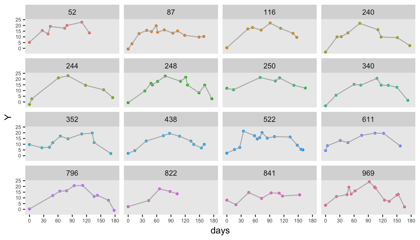
Here is a plot of the observed data for a sample of individuals:

Addendum

To verify that the data are indeed correlated with an AR-1 structure, I first convert the complete (latent) data from step 2 from its long format to a wide format. The correlation is calculated from this \(1000 \times 181\) matrix, where each row is an individual and each column is a value of \(Y\) at a different time point. And since the correlation matrix, which has dimensions \(181 \times 181\), is too big to show, what you see is only the upper left hand corner of the matrix:

round(cor(as.matrix(dcast(dtY, id ~ time, 
    value.var = "Y")[, -1]))[1:13, 1:13], 1)

##      0   1   2   3   4   5   6   7   8   9  10  11  12
## 0  1.0 0.4 0.2 0.1 0.0 0.0 0.1 0.0 0.0 0.0 0.1 0.0 0.0
## 1  0.4 1.0 0.4 0.1 0.0 0.0 0.0 0.0 0.0 0.0 0.0 0.0 0.0
## 2  0.2 0.4 1.0 0.4 0.2 0.1 0.0 0.0 0.1 0.0 0.0 0.0 0.0
## 3  0.1 0.1 0.4 1.0 0.4 0.2 0.1 0.0 0.0 0.0 0.0 0.0 0.1
## 4  0.0 0.0 0.2 0.4 1.0 0.4 0.2 0.1 0.0 0.1 0.0 0.0 0.0
## 5  0.0 0.0 0.1 0.2 0.4 1.0 0.4 0.2 0.1 0.0 0.0 0.0 0.0
## 6  0.1 0.0 0.0 0.1 0.2 0.4 1.0 0.4 0.2 0.0 0.0 0.0 0.0
## 7  0.0 0.0 0.0 0.0 0.1 0.2 0.4 1.0 0.4 0.2 0.1 0.1 0.0
## 8  0.0 0.0 0.1 0.0 0.0 0.1 0.2 0.4 1.0 0.4 0.1 0.0 0.0
## 9  0.0 0.0 0.0 0.0 0.1 0.0 0.0 0.2 0.4 1.0 0.4 0.2 0.0
## 10 0.1 0.0 0.0 0.0 0.0 0.0 0.0 0.1 0.1 0.4 1.0 0.4 0.2
## 11 0.0 0.0 0.0 0.0 0.0 0.0 0.0 0.1 0.0 0.2 0.4 1.0 0.4
## 12 0.0 0.0 0.0 0.1 0.0 0.0 0.0 0.0 0.0 0.0 0.2 0.4 1.0