I am involved with a stepped-wedge designed study that is exploring whether we can improve care for patients with end-stage disease who show up in the emergency room. The plan is to train nurses and physicians in palliative care. (A while ago, I described what the stepped wedge design is.)
Under this design, 33 sites around the country will receive the training at some point, which is no small task (and fortunately as the statistician, this is a part of the study I have little involvement). After hearing about this ambitious plan, a colleague asked why we didn’t just randomize half the sites to the intervention and conduct a more standard cluster randomized trial, where a site would either get the training or not. I quickly simulated some data to see what we would give up (or gain) if we had decided to go that route. (It is actually a moot point, since there would be no way to simultaneously train 16 or so sites, which is why we opted for the stepped-wedge design in the first place.)
I simplified things a bit by comparing randomization within site with randomization by site. The stepped wedge design is essentially a within-site randomization, except that the two treatment arms are defined at different time points, and things are complicated a bit because there might be time by intervention confounding. But, I won’t deal with that here.
Simulate data
library(simstudy)

# define data

cvar <- iccRE(0.20, dist = "binary")

d <- defData(varname = "a", formula = 0, variance = cvar,
               dist = "normal", id = "cid")
d <- defData(d, varname = "nper", formula = 100, dist = "nonrandom")

da <- defDataAdd(varname = "y", formula = "-1 + .4*rx + a",
                 dist="binary", link = "logit")
Randomize within cluster
set.seed(11265)

dc <- genData(100, d)

di <- genCluster(dc, "cid", "nper", "id")
di <- trtAssign(di, strata = "cid", grpName = "rx")
di <- addColumns(da, di)

di
## id rx cid a nper y
## 1: 1 1 1 -0.4389391 100 1
## 2: 2 0 1 -0.4389391 100 0
## 3: 3 1 1 -0.4389391 100 0
## 4: 4 0 1 -0.4389391 100 0
## 5: 5 0 1 -0.4389391 100 1
## ---
## 9996: 9996 0 100 -1.5749783 100 0
## 9997: 9997 1 100 -1.5749783 100 0
## 9998: 9998 0 100 -1.5749783 100 0
## 9999: 9999 1 100 -1.5749783 100 0
## 10000: 10000 1 100 -1.5749783 100 0I fit a conditional mixed effects model, and then manually calculate the conditional log odds from the data just to give a better sense of what the conditional effect is (see earlier post for more on conditional vs. marginal effects).
library(lme4)
rndTidy(glmer(y ~ rx + (1 | cid), data = di, family = binomial))
## term estimate std.error statistic p.value group
## 1 (Intercept) -0.86 0.10 -8.51 0 fixed
## 2 rx 0.39 0.05 8.45 0 fixed
## 3 sd_(Intercept).cid 0.95 NA NA NA cidcalc <- di[, .(estp = mean(y)), keyby = .(cid, rx)]
calc[, lo := log(odds(estp))]
calc[rx == 1, mean(lo)] - calc[rx == 0, mean(lo)] ## [1] 0.3985482Next, I fit a marginal model and calculate the effect manually as well.
library(geepack)
rndTidy(geeglm(y ~ rx, data = di, id = cid, corstr = "exchangeable",
            family = binomial))
## term estimate std.error statistic p.value
## 1 (Intercept) -0.74 0.09 67.09 0
## 2 rx 0.32 0.04 74.80 0log(odds(di[rx==1, mean(y)])/odds(di[rx==0, mean(y)]))## [1] 0.323471As expected, the marginal estimate of the effect is less than the conditional effect.
Randomize by cluster
Next we repeat all of this, though randomization is at the cluster level.
dc <- genData(100, d)
dc <- trtAssign(dc, grpName = "rx")

di <- genCluster(dc, "cid", "nper", "id")
di <- addColumns(da, di)

di
## cid rx a nper id y
## 1: 1 0 0.8196365 100 1 0
## 2: 1 0 0.8196365 100 2 1
## 3: 1 0 0.8196365 100 3 0
## 4: 1 0 0.8196365 100 4 0
## 5: 1 0 0.8196365 100 5 0
## ---
## 9996: 100 1 -0.1812079 100 9996 1
## 9997: 100 1 -0.1812079 100 9997 0
## 9998: 100 1 -0.1812079 100 9998 0
## 9999: 100 1 -0.1812079 100 9999 1
## 10000: 100 1 -0.1812079 100 10000 0Here is the conditional estimate of the effect:
rndTidy(glmer(y~rx + (1|cid), data = di, family = binomial))## term estimate std.error statistic p.value group
## 1 (Intercept) -0.71 0.15 -4.69 0.00 fixed
## 2 rx 0.27 0.21 1.26 0.21 fixed
## 3 sd_(Intercept).cid 1.04 NA NA NA cidAnd here is the marginal estimate
rndTidy(geeglm(y ~ rx, data = di, id = cid, corstr = "exchangeable",
            family = binomial))
## term estimate std.error statistic p.value
## 1 (Intercept) -0.56 0.13 18.99 0.00
## 2 rx 0.21 0.17 1.46 0.23While the within- and by-site randomization estimates are quite different, we haven’t really learned anything, since those differences could have been due to chance. So, I created 500 data sets under different assumptions to see what the expected estimate would be as well as the variability of the estimate.
Fixed ICC, varied randomization
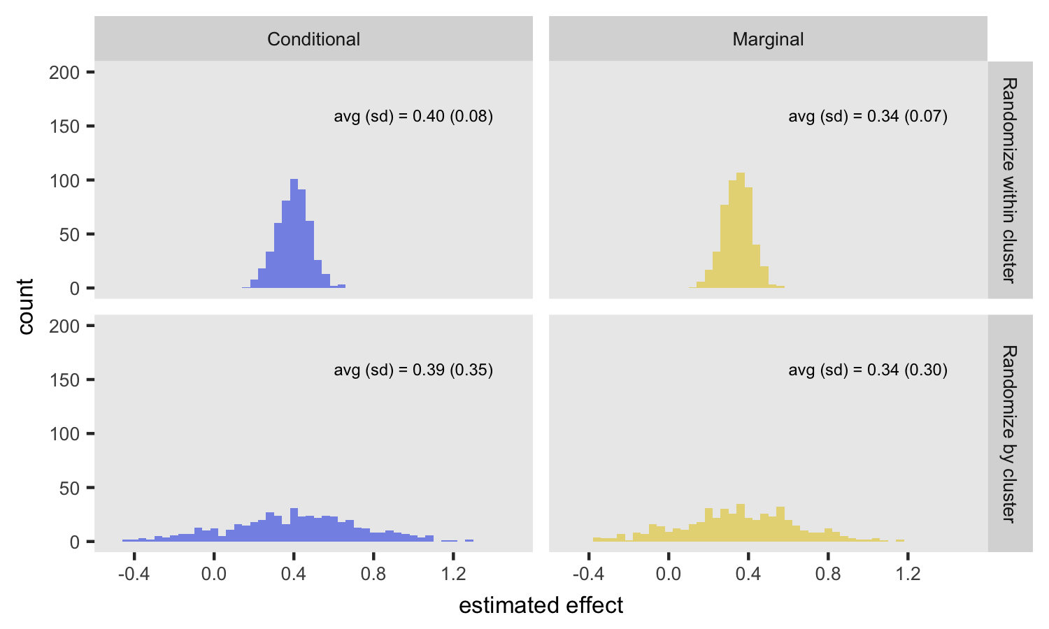
From this first set of simulations, the big take away is that randomizing within clusters provides an unbiased estimate of the conditional effect, but so does randomizing by site. The big disadvantage of randomizing by site is the added variability of the conditional estimate. The attenuation of the marginal effect estimates under both scenarios has nothing to do with randomization, but results from intrinsic variability across sites.

Fixed randomization, varied ICC
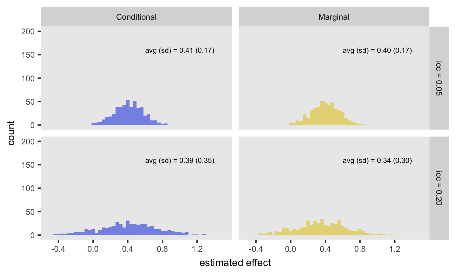
This next figure isolates the effect of across-site variability on the estimates. In this case, randomization is only by site (i.e. no within site randomization), but the ICC is set at 0.05 and 0.20. For the conditional model, the ICC has no impact on the expected value of the log-odds ratio, but when variability is higher (ICC = 0.20), the standard error of the estimate increases. For the marginal model, the ICC has an impact on both the expected value and standard error of the estimate. In the case with a low ICC (top row in plot), the marginal and condition estimates are quite similar.
