Be careful not to control for a post-exposure covariate

A researcher was presenting an analysis of the impact various types of childhood trauma might have on subsequent substance abuse in adulthood. Obviously, a very interesting and challenging research question. The statistical model included adjustments for several factors that are plausible confounders of the relationship between trauma and substance use, such as childhood poverty. However, the model also include a measurement for poverty in adulthood - believing it was somehow confounding the relationship of trauma and substance use. A confounder is a common cause of an exposure/treatment and an outcome; it is hard to conceive of adult poverty as a cause of childhood events, even though it might be related to adult substance use (or maybe not). At best, controlling for adult poverty has no impact on the conclusions of the research; less good, though, is the possibility that it will lead to the conclusion that the effect of trauma is less than it actually is.

Using a highly contrived simulation of data and the abstract concept of potential outcomes, I am hoping to illuminate some of the issues raised by this type of analysis.

Potential outcomes and causal effects

The field of causal inference is a rich one, and I won’t even scratch the surface here. My goal is to present the concepts of potential outcomes so that we can articulate at least one clear way to think about what a causal effect can be defined. Under this framework, we generate data where we can find out the “true” measure of causal effect. And then we can use simple regression models to see how well (or not) they recapture these “known” causal effects.

If an individual $i$ experiences a traumatic effect as a child, we say that the exposure $X_i = 1$ . Otherwise $X_i = 0$ , there was no traumatic event. (I am going to assume binary exposures just to keep things simple - exposed vs. not exposed.) In the potential outcomes world we say that every individual has possible outcomes $Y_{1i}$ (the outcome we would observe if the individual had experienced trauma) and $Y_{0i}$ (the outcome we would observe if the individual had not. Quite simply, we define the causal effect of $X$ on $Y$ as the difference in potential outcomes, $CE_i = Y_{1i} - Y_{0i}$ . If $Y_{1i} = Y_{0i}$ (i.e. the potential outcomes are the same), we would say that $X$ does not cause $Y$ , at least for individual $i$ .

In the real world, we only observe one potential outcome - the one associated with the actual exposure. The field of causal inference has lots to say about the assumptions and conditions that are required for us to use observed data to estimate average causal effects; many would say that unless we use a randomized controlled study, those assumptions will never be reasonable. But in the world of simulation, we can generate potential outcomes and observed outcomes, so we know the causal effect both at the individual level and the average population level. And we can see how well our models do.

Simple confounding

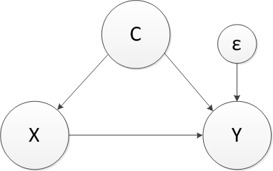
Here’s a relatively straightforward example. Let’s say we are interested in understanding if some measure $X$ causes an outcome $Y$ , where there is a common cause $C$ (the diagram is called a DAG - a directed acyclic graph - and is useful for many things, including laying out data generating process):

library(broom)
library(data.table)
library(simstudy)

def <- defData(varname = "C", formula = 0.4, dist = "binary")
def <- defData(def, "X", formula = "0.3 + 0.4 * C", dist = "binary")
def <- defData(def, "e", formula = 0, variance = 2, dist = "normal")
def <- defData(def, "Y0", formula = "2 * C + e", dist="nonrandom")
def <- defData(def, "Y1", formula = "0.5 + 2 * C + e", dist="nonrandom")
def <- defData(def, "Y_obs", formula = "Y0 + (Y1 - Y0) * X", dist = "nonrandom")

def

##    varname            formula variance      dist     link
## 1:       C                0.4        0    binary identity
## 2:       X      0.3 + 0.4 * C        0    binary identity
## 3:       e                  0        2    normal identity
## 4:      Y0          2 * C + e        0 nonrandom identity
## 5:      Y1    0.5 + 2 * C + e        0 nonrandom identity
## 6:   Y_obs Y0 + (Y1 - Y0) * X        0 nonrandom identity

In this example, $X$ does have an effect on $Y$ , but so does $C$ . If we ignore $C$ in assessing the size of the effect of $X$ on $Y$ , we will overestimate that effect, which is 0.5. We can generate data and see that this is the case:

set.seed(5)
dt <- genData(1000, def)

We see that the true causal effect is easily recovered if we have access to the potential outcomes $Y_1$ and $Y_0$ , but of course we don’t:

dt[, mean(Y1 - Y0)] # True causal effect

## [1] 0.5

If we compare the average observed outcomes for each exposure group ignoring the confounder, we overestimate the effect of the exposure:

dt[X == 1, mean(Y_obs)] - dt[X == 0, mean(Y_obs)]

## [1] 1.285009

We can estimate the same effect using simple linear regression:

lm1 <- lm(Y_obs ~ X, data = dt)
tidy(lm1)

## # A tibble: 2 x 5
##   term        estimate std.error statistic  p.value
##   <chr>          <dbl>     <dbl>     <dbl>    <dbl>
## 1 (Intercept)    0.552    0.0733      7.53 1.14e-13
## 2 X              1.29     0.107      12.0  2.92e-31

And finally, if we adjust for the confounder $C$ , we recover the true causal effect of $X$ on $Y$ , or at least get very close to it:

lm2 <- lm(Y_obs ~ X + C, data = dt)
tidy(lm2)

## # A tibble: 3 x 5
##   term        estimate std.error statistic  p.value
##   <chr>          <dbl>     <dbl>     <dbl>    <dbl>
## 1 (Intercept)   0.0849    0.0650      1.31 1.92e- 1
## 2 X             0.489     0.0968      5.06 5.08e- 7
## 3 C             2.06      0.0983     20.9  5.77e-81

Adjusting for a post-exposure covariate

Now, we are ready to see what happens in a slightly more complicated setting that is defined by this DAG:

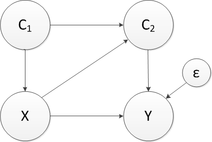
In this example $C$ is measured in two time periods, and exposure in period 1 relates to exposure in period 2. (For example, if a child is poor, he is more likely to be poor as an adult.) We are primarily interested in whether or not $X$ (trauma) causes $Y$ (substance use). The difficulty is that $X$ and $C_2$ are related, as are $C_2$ and $Y$ .

I suggest that in order to fully understand the effect of $X$ on $Y$ , we cannot control for $C_2$ , as tempting as it might be. The intuition is that part of the effect of $X$ on $Y$ is due to the fact that $X$ has an effect on $C_2$ , at least for some individuals. If we control for $C_2$ , we are actually removing a key component of the causal mechanism. Below in is the data generating process - a few things to note: (1) $C_2$ has potential outcomes based on the exposure $X$ . (2) We have restricted the potential outcome $C_{21}$ to be set to 1 if $C_{20}$ is 1. For example, if someone would have been poor in adulthood without exposure to trauma, we assume that they also would have been poor in adulthood had they been exposed to trauma. (3) The potential outcome for $Y$ is dependent on the relevant potential outcome for $C_2$ . That is $Y_0$ depends on $C_{20}$ and $Y_1$ depends on $C_{21}$ .

def2 <- defData(varname = "C1", formula = .25, dist = "binary")
def2 <- defData(def2, "X", formula = "-2 + 0.8 * C1", dist = "binary", link = "logit")
def2 <- defData(def2, "C2.0", formula = "-2.0 + 1 * C1", dist = "binary", link = "logit")
def2 <- defData(def2, "C2.1x", formula = "-1.5 + 1 * C1", dist = "binary", link = "logit")
def2 <- defData(def2, "C2.1", formula = "pmax(C2.0, C2.1x)", dist = "nonrandom")
def2 <- defData(def2, "e", formula = 0, variance = 4, dist = "normal")
def2 <- defData(def2, "Y0", formula = "-3 + 5*C2.0 + e", dist = "nonrandom")
def2 <- defData(def2, "Y1", formula = "0 + 5*C2.1 + e", dist = "nonrandom")
def2 <- defData(def2, "C2_obs", formula = "C2.0 + (C2.1 - C2.0) * X", dist = "nonrandom")
def2 <- defData(def2, "Y_obs", formula = "Y0 + (Y1 - Y0) * X", dist = "nonrandom")

set.seed(25)
dt <- genData(5000, def2)

Here is the true average causal effect, based on information we will never know:

dt[, mean(Y1 - Y0)]

## [1] 3.903

When we control for $C_2$ , we are essentially estimating the effect of $X$ at each level $C_2$ (and $C_1$ , since we are controlling for that as well), and then averaging across the sub-samples to arrive at an estimate for the entire sample. We can see that, based on the specification of the potential outcomes in the data generation process, the effect at each level of $C_2$ will be centered around 3.0, which is different from the true causal effect of 3.9. The discrepancy is due to the fact each approach is effectively collecting different sub-samples (one defines groups based on set levels of $X$ and $C_2$ , and the other defines groups based on set levels of $X$ alone) and estimating average effects based on weights determined by the sizes of those two sets of sub-samples.

Here is the inappropriate model that adjusts for $C_2$ :

lm2a <- lm( Y_obs ~ C1 + C2_obs + X , data = dt)
tidy(lm2a)

## # A tibble: 4 x 5
##   term        estimate std.error statistic   p.value
##   <chr>          <dbl>     <dbl>     <dbl>     <dbl>
## 1 (Intercept)  -3.01      0.0348   -86.6   0.       
## 2 C1           -0.0208    0.0677    -0.307 7.59e-  1
## 3 C2_obs        4.93      0.0763    64.6   0.       
## 4 X             3.05      0.0811    37.5   6.68e-272

The estimate for the coefficient of $X$ is 3.0, just as anticipated. Here now is the correct model, and you will see that we recover the true causal effect in the coefficient estimate of $X$ (or at least, we get much, much closer):

lm2b <- lm( Y_obs ~ C1 + X , data = dt)
tidy(lm2b)

## # A tibble: 3 x 5
##   term        estimate std.error statistic   p.value
##   <chr>          <dbl>     <dbl>     <dbl>     <dbl>
## 1 (Intercept)   -2.49     0.0459     -54.3 0.       
## 2 C1             0.967    0.0893      10.8 5.32e- 27
## 3 X              3.94     0.108       36.3 7.87e-257

Of course, in the real world, we don’t know the underlying data generating process or the true DAG. And what I have described here is a gross oversimplification of the underlying relationships, and have indeed left out many other factors that likely affect the relationship between childhood trauma and adult substance use. Other measures, such as parental substance use, may be related to both childhood trauma and adult substance use, and may affect poverty in the two time periods in different, complicated ways.

But the point is that one should give careful thought to what gets included in a model. We may not want to throw everything we measure into the model. Be careful.