It is grant season around here (actually, it is pretty much always grant season), which means another series of problems to tackle. Even with the most straightforward study designs, there is almost always some interesting twist, or an approach that presents a subtle issue or two. In this case, the investigator wants compare two interventions, but doesn’t feel the need to show that one is better than the other. He just wants to see if the newer intervention is not inferior to the more established intervention.
The shift from a superiority trial to a non-inferiority trial leads to a fundamental shift in the hypothesis testing framework. In the more traditional superiority trial, where we want to see if an intervention is an improvement over another intervention, we can set up the hypothesis test with null and alternative hypotheses based on the difference of the intervention proportions \(p_{old}\) and \(p_{new}\) (under the assumption of a binary outcome):
\[ \begin{aligned} H_0: p_{new} - p_{old} &\le 0 \\ H_A: p_{new} - p_{old} &> 0 \end{aligned} \] In this context, if we reject the null hypothesis that the difference in proportions is less than zero, we conclude that the new intervention is an improvement over the old one, at least for the population under study. (A crucial element of the test is the \(\alpha\)-level that determines the Type 1 error (probability of rejecting \(H_0\) when \(H_0\) is actually true. If we use \(\alpha = 0.025\), then that is analogous to doing a two-sided test with \(\alpha = .05\) and hypotheses \(H_0: p_{new} - p_{old} = 0\) and \(H_A: p_{new} - p_{old} \neq 0\).)
In the case of an inferiority trial, we add a little twist. Really, we subtract a little twist. In this case the hypotheses are:
\[ \begin{aligned} H_0: p_{new} - p_{old} &\le -\Delta \\ H_A: p_{new} - p_{old} &> -\Delta \end{aligned} \]
where \(\Delta\) is some threshold that sets the non-inferiority bounds. Clearly, if \(\Delta = 0\) then this is equivalent to a superiority test. However, for any other \(\Delta\) there is a bit of a cushion so that the new intervention will still be considered non-inferior even if we observe a lower proportion for the new intervention compared to the older intervention.
As long as the confidence interval around the observed estimate for the difference in proportions does not cross the \(-\Delta\) threshold, we can conclude the new intervention is non-inferior. If we construct a 95% confidence interval, this procedure will have a Type 1 error rate \(\alpha = 0.025\), and a 90% CI will yield an \(\alpha = 0.05\). (I will demonstrate this with a simulation.)
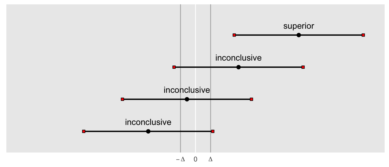
The following figures show how different confident intervals imply different conclusions. I’ve added an equivalence trial here as well, but won’t discuss in detail except to say that in this situation we would conclude that two interventions are equivalent if the confidence interval falls between \(-\Delta\) and \(\Delta\)). The bottom interval crosses the non-inferiority threshold, so is considered inconclusive. The second interval from the top crosses zero, but does not cross the non-inferiority threshold, so we conclude that the new intervention is at least as effective as the old one. And the top interval excludes zero, so we conclude that the new intervention is an improvement:

This next figure highlights the key challenge of the the non-inferiority trial: where do we set \(\Delta\)? By shifting the threshold towards zero in this example (and not changing anything else), we can no longer conclude non-inferiority. But, the superiority test is not affected, and never will be. The comparison for a superiority test is made relative to zero only, and has nothing to do with \(\Delta\). So, unless there is a principled reason for selecting \(\Delta\), the process (and conclusions) can feel a little arbitrary. (Check out this interactive post for a really cool way to explore some of these issues.)

Type 1 error rate
To calculate the Type 1 error rate, we generate data under the null hypothesis, or in this case on the rightmost boundary of the null hypothesis since it is a composite hypothesis. First, let’s generate one data set:
library(magrittr)
library(broom)

set.seed(319281)

def <- defDataAdd(varname = "y", formula = "0.30 - 0.15*rx",
                  dist = "binary")

DT <- genData(1000) %>% trtAssign(dtName = ., grpName = "rx")
DT <- addColumns(def, DT)
DT
## id rx y
## 1: 1 1 1
## 2: 2 0 0
## 3: 3 0 0
## 4: 4 0 1
## 5: 5 0 0
## ---
## 996: 996 0 0
## 997: 997 0 0
## 998: 998 0 0
## 999: 999 1 0
## 1000: 1000 1 0And we can estimate a confidence interval for the difference between the two means:
props <- DT[, .(success = sum(y), n=.N), keyby = rx]
setorder(props, -rx)

round(tidy(prop.test(props$success, props$n,
               correct = FALSE, conf.level = 0.95))[ ,-c(5, 8,9)], 3)
## # A tibble: 1 × 6
## estimate1 estimate2 statistic p.value conf.low conf.high
## <dbl> <dbl> <dbl> <dbl> <dbl> <dbl>
## 1 0.16 0.234 8.65 0.003 -0.123 -0.025If we generate 1000 data sets in the same way, we can count the number of occurrences where the where we would incorrectly reject the null hypothesis (i.e. commit a Type 1 error):
powerRet <- function(nPerGrp, level, effect, d = NULL) {

  Form <- genFormula(c(0.30, -effect), c("rx"))

  def <- defDataAdd(varname = "y", formula = Form, dist = "binary")
  DT <- genData(nPerGrp*2) %>% trtAssign(dtName = ., grpName = "rx")

  iter <- 1000
  ci <- data.table()

  # generate 1000 data sets and store results each time in "ci"

  for (i in 1: iter) {

    dx <- addColumns(def, DT)

    props <- dx[, .(success = sum(y), n=.N), keyby = rx]
    setorder(props, -rx)
    ptest <- prop.test(props$success, props$n, correct = FALSE,
                       conf.level = level)

    ci <- rbind(ci, data.table(t(ptest$conf.int),
                       diff = ptest$estimate[1] - ptest$estimate[2]))
  }

  setorder(ci, V1)
  ci[, i:= 1:.N]

  # for sample size calculation at 80% power

  if (is.null(d)) d <- ci[i==.2*.N, V1]

  ci[, d := d]

  # determine if interval crosses threshold

  ci[, nullTrue := (V1 <= d)]

  return(ci[])

}
Using 95% CIs, we expect 2.5% of the intervals to lie to the right of the non-inferiority threshold. That is, 2.5% of the time we would reject the null hypothesis when we shouldn’t:
ci <- powerRet(nPerGrp = 500, level = 0.95, effect = 0.15, d = -0.15)
formattable::percent(ci[, mean(!(nullTrue))], 1)
## [1] 2.4%And using 90% CIs, we expect 5% of the intervals to lie to the right of the threshold:
ci <- powerRet(nPerGrp = 500, level = 0.90, effect = 0.15, d = -0.15)
formattable::percent(ci[, mean(!(nullTrue))], 1)
## [1] 4.8%Sample size estimates
If we do not expect the effect sizes to be different across interventions, it seems reasonable to find the sample size under this assumption of no effect. Assuming we want to set \(\alpha = 0.025\), we generate many data sets and estimate the 95% confidence interval for each one. The power is merely the proportion of these confidence intervals lie entirely to the right of \(-\Delta\).
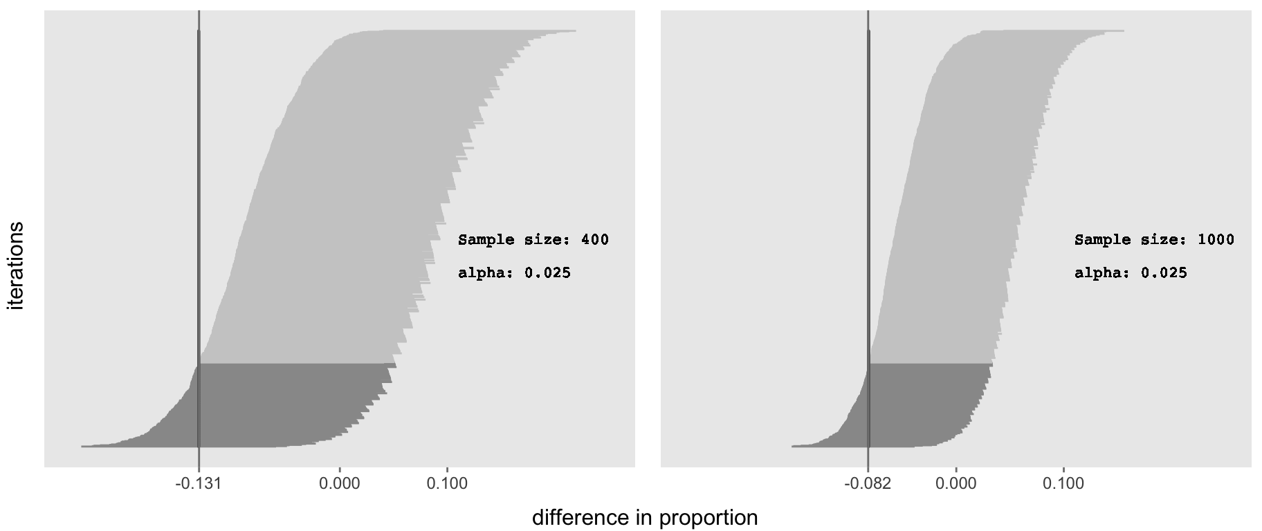
But how should we set \(\Delta\)? I’d propose that for each candidate sample size level, we find \(-\Delta\) such that 80% of the simulated confidence intervals lie to the right of some value, where 80% is the desired power of the test (i.e., given that there is no treatment effect, 80% of the (hypothetical) experiments we conduct will lead us to conclude that the new treatment is non-inferior to the old treatment).
ci <- powerRet(nPerGrp = 200, level = 0.95, effect = 0)
p1 <- plotCIs(ci, 200, 0.95)

ci <- powerRet(nPerGrp = 500, level = 0.95, effect = 0)
p2 <- plotCIs(ci, 500, 0.95)
library(gridExtra)
grid.arrange(p1, p2, nrow = 1,
bottom = "difference in proportion", left = "iterations")
It is clear that increasing the sample size reduces the width of the 95% confidence intervals. As a result, the non-inferiority threshold based on 80% power is shifted closer towards zero when sample size increases. This implies that a larger sample size allows us to make a more compelling statement about non-inferiority.
Unfortunately, not all non-inferiority statements are alike. If we set \(\Delta\) too large, we may expand the bounds of non-inferiority beyond a reasonable, justifiable point. Given that there is no actual constraint on what \(\Delta\) can be, I would say that the non-inferiority test is somewhat more problematic than its closely related cousin, the superiority test, where \(\Delta\) is in effect fixed at zero. But, if we take this approach, where we identify \(\Delta\) that satisfies the desired power, we can make a principled decision about whether or not the threshold is within reasonable bounds.