Modeling data without any underlying causal theory can sometimes lead you down the wrong path, particularly if you are interested in understanding the way things work rather than making predictions. A while back, I described what can go wrong when you control for a mediator when you are interested in an exposure and an outcome. Here, I describe the potential biases that are introduced when you inadvertently control for a variable that turns out to be a collider.
A collider, like a mediator, is a post-exposure/post-intervention outcome. Unlike a mediator, a collider is not necessarily causally related to the outcome of interest. (This is not to say that it cannot be, which is why this concept came up in a talk I gave about marginal structural models, described here, here, and here.) The key distinction of a collider is that it is an outcome that has two causes. In a directed acyclic graph (or DAG), a collider is a variable with two arrows pointing towards it. This is easier to see visually:
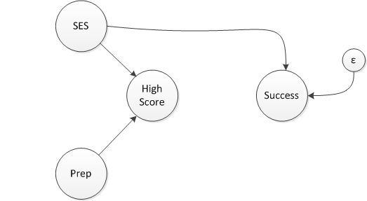
In this (admittedly thoroughly made-up though not entirely implausible) network diagram, the test score outcome is a collider, influenced by a test preparation class and socio-economic status (SES). In particular, both the test prep course and high SES are related to the probability of having a high test score. One might expect an arrow of some sort to connect SES and the test prep class; in this case, participation in test prep is randomized so there is no causal link (and I am assuming that everyone randomized to the class actually takes it, a compliance issue I addressed in a series of posts starting with this one.)
The researcher who carried out the randomization had a hypothesis that test prep actually is detrimental to college success down the road, because it de-emphasizes deep thinking in favor of wrote memorization. In reality, it turns out that the course and subsequent college success are not related, indicated by an absence of a connection between the course and the long term outcome.
Simulate data
We can simulate data from this hypothetical world (using functions from package simstudy):
# define data

library(simstudy)

defCollide <- defData(varname = "SES",
                      formula = "0;1",
                      dist = "uniform")

defCollide <- defData(defCollide, varname = "testPrep",
                      formula = 0.5,
                      dist = "binary")

defCollide <- defData(defCollide, varname = "highScore",
                      formula = "-1.2 + 3*SES + 3*testPrep",
                      dist = "binary", link="logit")

defCollide <- defData(defCollide, varname = "successMeasure",
                      formula = "20 + SES*40", variance = 9,
                      dist = "normal")

defCollide
## varname formula variance dist link
## 1: SES 0;1 0 uniform identity
## 2: testPrep 0.5 0 binary identity
## 3: highScore -1.2 + 3*SES + 3*testPrep 0 binary logit
## 4: successMeasure 20 + SES*40 9 normal identity# generate data
set.seed(139)
dt <- genData(1500, defCollide)
dt[1:6]## id SES testPrep highScore successMeasure
## 1: 1 0.52510665 1 1 40.89440
## 2: 2 0.31565690 0 1 34.72037
## 3: 3 0.47978492 1 1 41.79532
## 4: 4 0.19114934 0 0 30.05569
## 5: 5 0.06889896 0 0 21.28575
## 6: 6 0.10139604 0 0 21.30306We can see that the distribution of the long-term (continuous) success outcome is the same for those who are randomized to test prep compared to those who are not, indicating there is no causal relationship between the test and the college outcome:
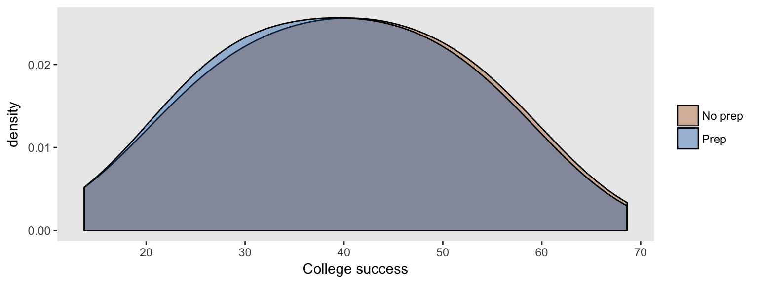
An unadjusted linear model leads us to the same conclusion, since the parameter estimate representing the treatment effect is quite small (and the hypothesis test is not statistically significant):
library(broom)

rndtidy( lm(successMeasure ~ testPrep, data = dt))
## term estimate std.error statistic p.value
## 1 (Intercept) 40.112 0.44 91.209 0.000
## 2 testPrep -0.495 0.61 -0.811 0.418But, don’t we need to adjust for some measure of intellectual ability?
Or so the researcher might ask after looking at the initial results, questioning the model. He believes that differences in ability could be related to future outcomes. While this may be the case, the question isn’t about ability but the impact of test prep. Based on his faulty logic, the researcher decides to fit a second model and control for the test score that followed the experiment. And this is where things go awry. Take a look at the following model where there appears to be a relationship between test prep and college success after controlling for the test score:
# adjusted model

rndtidy( lm(successMeasure ~ highScore + testPrep, data = dt))
## term estimate std.error statistic p.value
## 1 (Intercept) 35.525 0.619 57.409 0
## 2 highScore 8.027 0.786 10.207 0
## 3 testPrep -3.564 0.662 -5.380 0It does indeed appear that the test prep course is causing problems for real learning in college later on!
What is going on?
Because the test score (here I am treating it as binary - either a high score or not), is related to both SES and test prep, the fact that someone does well on the test is due either to the fact that the student took the course, has high SES, or both. But, let’s consider the students who are possibly high SES or maybe took the course, but not not both, and who had a high test score. If a student is low SES, she probably took the course, or if she did not take the course, she is probably high SES. So, within the group that scored well, SES and the probability of taking the course are slightly negatively correlated.
If we “control” for test scores in the model, we are essentially comparing students within two distinct groups - those who scored well and those who did not. The updated network diagram shows a relationship between SES and test prep that didn’t exist before. This is the induced relationship we get by controlling a collider. (Control is shown in the diagram by removing the connection of SES and test prep to the test score.)
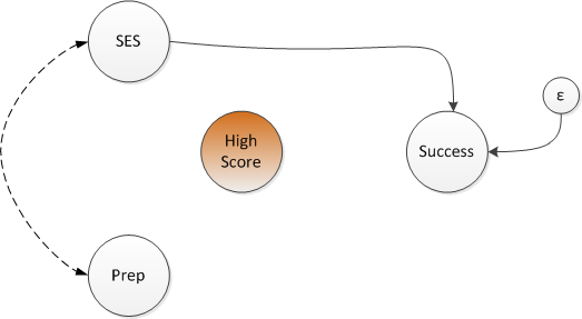
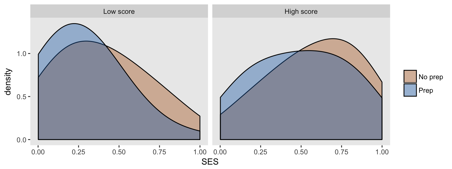
If we look at the entire sample and compare the SES distribution (which is a continuous measure uniformly distributed between 0 and 1) for each test prep group, we see that both groups have the same distribution (i.e. there is no relationship):
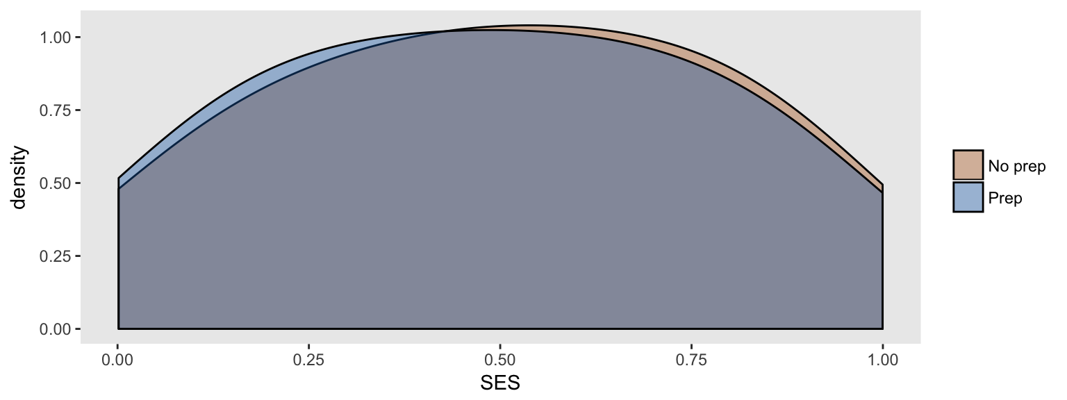
But if we look at the relationship between SES and test prep within each test score group, the distributions no longer completely overlap - within each test score group, there is a relationship between SES and test prep.
Why does this matter?
If the researcher has no good measure for SES or no measure at all, he cannot control for SES in the model. And now, because of the induced relationship between test prep and (unmeasured) SES, there is unmeasured confounding. This confounding leads to the biased estimate that we saw in the second model. And we see this bias in the densities shown for each test score group:
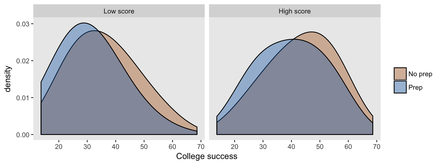
If it turns out that we can control for SES as well, because we have an adequate measure for it, then the artificial link between SES and test prep is severed, and so is the relationship between test prep and the long term college outcome.
rndtidy( lm(successMeasure ~ SES + highScore + testPrep, data = dt))## term estimate std.error statistic p.value
## 1 (Intercept) 19.922 0.194 102.519 0.000
## 2 SES 40.091 0.279 143.528 0.000
## 3 highScore -0.098 0.212 -0.462 0.644
## 4 testPrep 0.137 0.174 0.788 0.431The researcher can create problems by controlling for all the variables he has and not controlling for the variables he doesn’t have. Of course, if there are no colliders and mediators, then there is no harm. And unfortunately, without theory, it may be hard to know the structure of the DAG, particularly if there are important unmeasured variables. But, the researcher needs to proceed with a bit of caution.
Addendum: selection bias
“Selection bias” is used in a myriad of ways to characterize the improper assessment of an exposure-outcome relationship. For example, unmeasured confounding (where there is an unmeasured factor that influences both an exposure and an outcome) is often called selection bias, in the sense that the exposure is “selected” based on that particular characteristic.
Epidemiologists talk about selection bias in a very specific way, related to how individuals are selected or self-select into a study. In particular, if selection into a study depends on the exposure of interest and some other factor that is associated with the outcome, we can have selection bias.
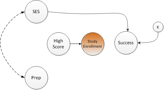
How is this relevant to this post? Selection bias results from controlling a collider. In this case, however, control is done on through the study design, rather than through statistical modeling. Let’s say we have the same scenario with a randomized trial of a test prep course and we are primarily interested in the impact on the near-term test score. But, later on, we decide to explore the relationship of the course with the long-term college outcome and we send out a survey to collect the college outcome data. It turns out that those who did well on the near-term test were much more likely to respond to the survey - so those who have been selected (or in this case self-selected) will have an induced relationship between the test prep course and SES, just as before. Here is the new DAG:
Simulate new study selection variable
The study response or selection variable is dependent on the near-term test score. The selected group is explicitly defined by the value of inStudy
# selection bias

defS <- defDataAdd(varname = "inStudy",
                   formula = "-2.0 + 2.2 * highScore",
                   dist = "binary", link = "logit")

dt <- addColumns(defS, dt)

dSelect <- dt[inStudy == 1]
We can see that a large proportion of the the selected group has a high probability of having scored high on the test score:
dSelect[, mean(highScore)]## [1] 0.9339207Selection bias is a muted version of full-on collider bias
Within this group of selected students, there is an (incorrectly) estimated relationship between the test prep course and subsequent college success. This bias is what epidemiologists are talking about when they talk about selection bias:
rndtidy( lm(successMeasure ~ testPrep, data = dSelect))## term estimate std.error statistic p.value
## 1 (Intercept) 41.759 0.718 58.154 0.000
## 2 testPrep -2.164 0.908 -2.383 0.017