Just before heading out on vacation last month, I put up a post that purported to compare stepped-wedge study designs with more traditional cluster randomized trials. Either because I rushed or was just lazy, I didn’t exactly do what I set out to do. I did confirm that a multi-site randomized clinical trial can be more efficient than a cluster randomized trial when there is variability across clusters. (I compared randomizing within a cluster with randomization by cluster.) But, this really had nothing to with stepped-wedge designs.
Here, I will try to rectify the shortcomings of that post by actually simulating data from a traditional stepped-wedge design and two variations on that theme with the aim of seeing which approach might be preferable. These variations were inspired by this extremely useful paper by Thompson et al. (If you stop reading here and go to the paper, I will consider mission accomplished.)
The key differences in the various designs are how many sites are exposed to the intervention and what the phase-in schedule looks like. In the examples that follow, I am assuming a study that lasts 24 weeks and with 50 total sites. Each site will include six patients per week. That means if we are collecting data for all sites over the entire study period, we will have outcome measurements.
The most important assumption I am making, however, is that the investigators can introduce the intervention at a small number of sites during each time period (for example, because the intervention involves extensive training and there is a limited number of trainers.) In this case, I am assuming that at most 10 sites can start the intervention at any point in time, and we must wait at least 4 weeks until the next wave can be started. (We can proceed slower than 4 weeks, of course, which surprisingly may be the best option.)
I am going to walk through the data generation process for each of the variations and then present the results of a series of power analyses to compare and contrast each design.
Stepped-wedge design

In the stepped-wedge design, all clusters in a trial will receive the intervention at some point, but the start of the intervention will be staggered. The amount of time in each state (control or intervention) will differ for each site (or group of sites if there are waves of more than one site starting up at the same time).
In this design (and in the others as well) time is divided into discrete data collection/phase-in periods. In the schematic figure, the light blue sections are periods during which the sites are in a control state, and the darker blue are periods during which the sites are in the intervention state. Each period in this case is 4 weeks long.
Following the Thompson et al. paper, the periods can be characterized as pre-rollout (where no intervention occurs), rollout (where the intervention is introduced over time), and post-rollout (where the all clusters are under intervention). Here, the rollout period includes periods two through five.
First, we define the data, which will largely be the same across the designs: 6 individual patients per week, an intervention effect of 0.33, and a weekly time effect (which unfortunately is parameterized as “period”) of 0.02, and standard deviation within each cluster of 3.
library(simstudy)

defS <- defData(varname = "n", formula = 6,
                dist = "nonrandom", id = "site")
defS <- defData(defS, varname = "siteInt", formula = 0,
                variance = 1, dist = "normal")

defP <- defDataAdd(varname = "rx",
                   formula = "(start <= period) * everTrt",
                   dist = "nonrandom")

defI <- defDataAdd(varname = "Y",
                   formula = "10 + rx * 0.33 + period * 0.02 + siteInt",
                   variance = 9, dist = "normal")
Now, we actually generate the data, starting with the site level data, then the period data, and then the individual patient level data. Note that the intervention is phased in every 4 weeks so that by the end of the 24 weeks all 5 waves are operating under the intervention:
set.seed(111)

dS <- genData(50, defS)
dS[, start := rep((1:5)*4, each = 10)]
dS[, everTrt := 1]

dS[site %in% c(1, 2, 11, 12, 49, 50)] # review a subset
## site n siteInt start everTrt
## 1: 1 6 0.2352207 4 1
## 2: 2 6 -0.3307359 4 1
## 3: 11 6 -0.1736741 8 1
## 4: 12 6 -0.4065988 8 1
## 5: 49 6 2.4856616 20 1
## 6: 50 6 1.9599817 20 1# weekly data
dP <- addPeriods(dtName = dS, nPeriods = 24, idvars = "site")
dP <- addColumns(defP, dP)
dP[site %in% c(3, 17) & period < 5] # review a subset## site period n siteInt start everTrt timeID rx
## 1: 3 0 6 -0.31162382 4 1 49 0
## 2: 3 1 6 -0.31162382 4 1 50 0
## 3: 3 2 6 -0.31162382 4 1 51 0
## 4: 3 3 6 -0.31162382 4 1 52 0
## 5: 3 4 6 -0.31162382 4 1 53 1
## 6: 17 0 6 -0.08585101 8 1 385 0
## 7: 17 1 6 -0.08585101 8 1 386 0
## 8: 17 2 6 -0.08585101 8 1 387 0
## 9: 17 3 6 -0.08585101 8 1 388 0
## 10: 17 4 6 -0.08585101 8 1 389 0# patient data
dI <- genCluster(dtClust = dP, cLevelVar = "timeID", numIndsVar = "n",
level1ID = "id")
dI <- addColumns(defI, dI)
dI## site period n siteInt start everTrt timeID rx id Y
## 1: 1 0 6 0.2352207 4 1 1 0 1 10.810211
## 2: 1 0 6 0.2352207 4 1 1 0 2 14.892854
## 3: 1 0 6 0.2352207 4 1 1 0 3 12.977948
## 4: 1 0 6 0.2352207 4 1 1 0 4 11.311097
## 5: 1 0 6 0.2352207 4 1 1 0 5 10.760508
## ---
## 7196: 50 23 6 1.9599817 20 1 1200 1 7196 11.317432
## 7197: 50 23 6 1.9599817 20 1 1200 1 7197 7.909369
## 7198: 50 23 6 1.9599817 20 1 1200 1 7198 13.048293
## 7199: 50 23 6 1.9599817 20 1 1200 1 7199 17.625904
## 7200: 50 23 6 1.9599817 20 1 1200 1 7200 7.147883Here is a plot of the site level averages at each time point:
library(ggplot2)

dSum <- dI[, .(Y = mean(Y)), keyby = .(site, period, rx, everTrt, start)]

ggplot(data = dSum, aes(x = period, y = Y, group = interaction(site, rx))) +
  geom_line(aes(color = factor(rx))) +
  facet_grid(factor(start, labels = c(1 : 5)) ~ .) +
  scale_x_continuous(breaks = seq(0, 23, by = 4), name = "week") +
  scale_color_manual(values = c("#b8cce4", "#4e81ba")) +
  theme(panel.grid = element_blank(),
legend.position = "none") 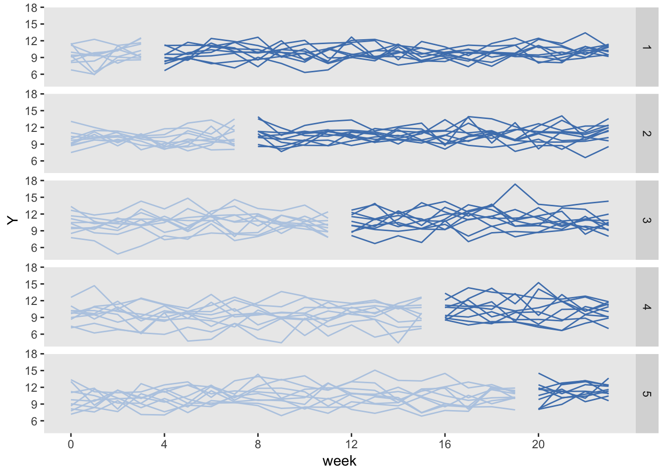
Finally, we can fit a linear mixed effects model to estimate the treatment effect:
library(lme4)
library(broom)

tidy(lmer(Y ~ rx + period + (1|site), data = dI))
## term estimate std.error statistic group
## 1 (Intercept) 9.78836231 0.184842722 52.955086 fixed
## 2 rx 0.35246094 0.122453829 2.878317 fixed
## 3 period 0.02110481 0.007845705 2.689983 fixed
## 4 sd_(Intercept).site 1.21303055 NA NA site
## 5 sd_Observation.Residual 2.99488532 NA NA ResidualStepped-wedge using “rollout” stage only

The Thompson et al. paper argued that if we limit the study to the rollout period only (periods 2 through 5 in the example above) but increase the length of the periods (here, from 4 to 6 weeks), we can actually increase power. In this case, there will be one wave of 10 sites that never receives the intervention.
The data generation process is exactly the same as above, except the statement defining the length of periods (6 weeks instead of 4 weeks) and starting point (week 0 vs. week 4) is slightly changed:
dS[, start := rep((0:4)*6, each = 10)]So the site level data set with starting points at 0, 6, 12, and 18 weeks for each of the four waves that ever receive treatment looks like this:
##    site n    siteInt start everTrt
## 1:    1 6  0.2352207     0       1
## 2:    2 6 -0.3307359     0       1
## 3:   11 6 -0.1736741     6       1
## 4:   12 6 -0.4065988     6       1
## 5:   49 6  2.4856616    24       1
## 6:   50 6  1.9599817    24       1
And the data generated under this scenario looks like:
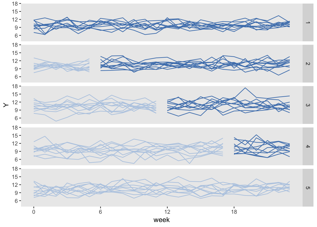
Here is the model estimation:
tidy(lmer(Y ~ rx + period + (1|site), data = dI))## term estimate std.error statistic group
## 1 (Intercept) 9.79022407 0.185294936 52.835897 fixed
## 2 rx 0.30707559 0.122414620 2.508488 fixed
## 3 period 0.02291619 0.006378367 3.592800 fixed
## 4 sd_(Intercept).site 1.21153700 NA NA site
## 5 sd_Observation.Residual 2.99490926 NA NA ResidualStaggered cluster randomized trial
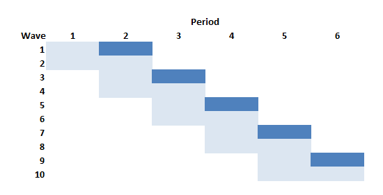
If we wanted to conduct a cluster randomized trial but were able to phase in the intervention over time as we have been assuming, this design is the closest we could get. In this example with 50 sites and five phase-in periods, the intervention waves (in this example 1, 3, 5, 7, and 9) would each include five clusters. The respective control waves (2, 4, 6, 8, and 10) would also have five clusters each. And since we are assuming five waves, each wave will be in the study for eight: the first four weeks comprise “pre” measurement period, and the second four week period is the “post” measurement period.
The problem with this design relative to all the others discussed here is that the amount of data collected for each site is considerably reduced. As a result, this design is going to be much less efficient (hence less powerful) than the others. So much so, that I do not even generate data for this design (though I did actually confirm using simulations not shown here.)
Staggered cluster randomized trial with continued measurement
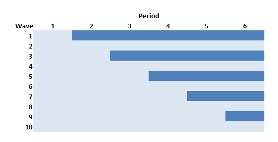
This is the staggered CRT just described, but we collect data for all 24 weeks for all of the sites. In this case, we are not at disadvantage with respect to the number of measurements, so it might be a competitive design. This version of staggered CRT could also be viewed as a traditional stepped-wedge design with controls.
The data generation is identical to the traditional stepped-wedge design we started with, except the only half of the sites are “ever treated”:
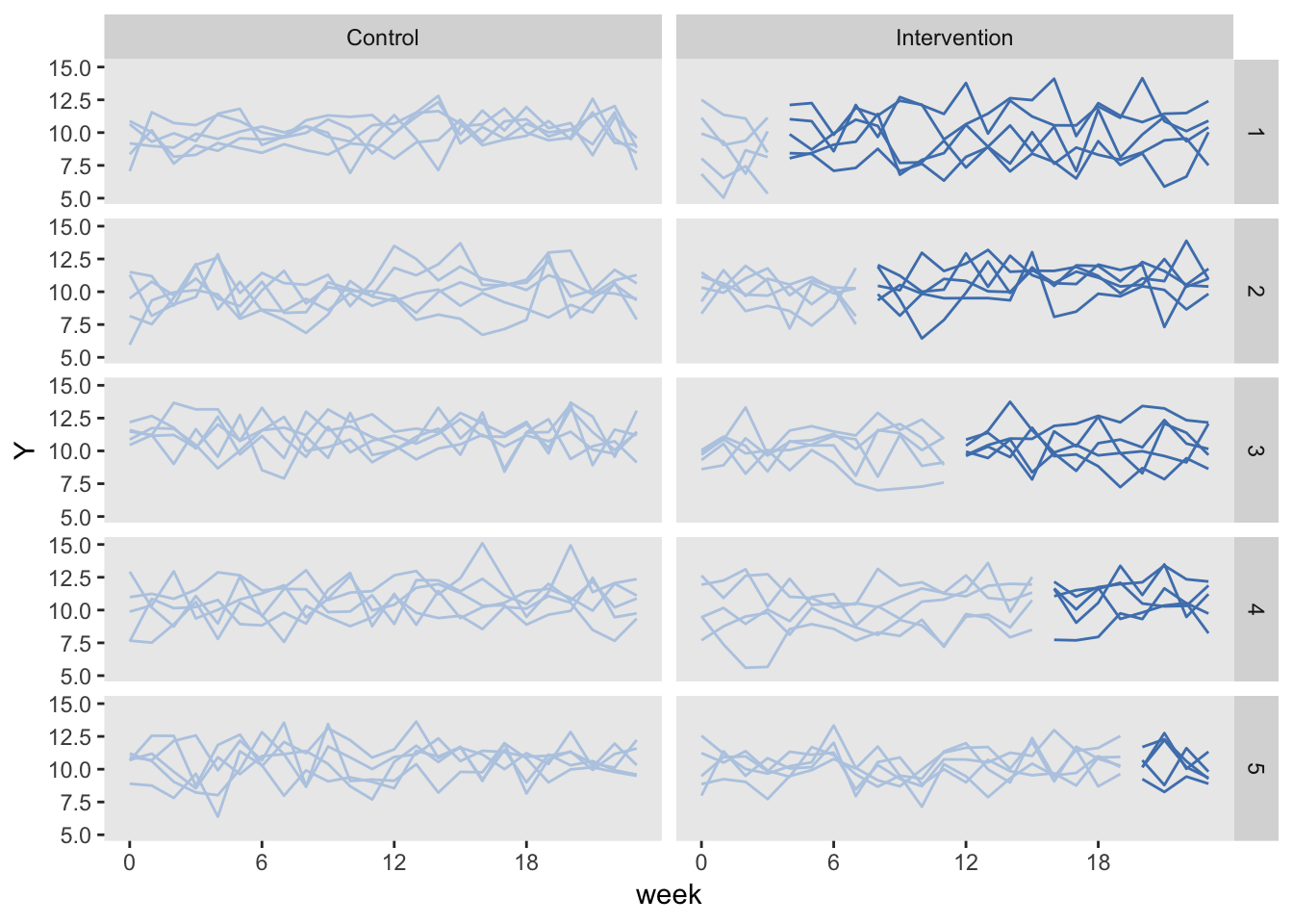
dS[, everTrt := rep(0:1)]Here is the plot, with the control arm on the left, and the intervention arm on the right. The control arm is never introduced to the intervention.
Conducting a power analysis using simulation
We are ultimately interested in assessing how much information each study design can provide. Power analyses under different conditions are one way to measure this.
Since one of my missions here is to illustrate as much R code as possible, here is how I do conduct the power analysis of the traditional stepped-wedge design:
powerStepWedge1 <- function(x) {

  # generate data

  dS <- genData(50, defS)
  dS[, start := rep((1:5)*4, each = 10)]
  dS[, everTrt := 1]

  dP <- addPeriods(dtName = dS, nPeriods = 24, idvars = "site")
  dP <- addColumns(defP, dP)

  dI <- genCluster(dtClust = dP, cLevelVar = "timeID",
                   numIndsVar = "n", level1ID = "id")
  dI <- addColumns(defI, dI)

  # fit model

  data.frame(summary(lmer(Y ~ rx + period + (1|site), data = dI))$coef)
}

res <- vector("list", length = 5)
i <- 0

for (icc in seq(0, 0.04, .01)) {

  i <- i + 1

  # update data definition based on new ICC

  between.var <- iccRE(ICC = icc, dist = "normal", varWithin = 9)
  defS <- updateDef(defS, changevar = "siteInt", newvariance = between.var)

  # generate 200 data sets and fit models
  resSW1<- lapply(1:200, FUN = powerStepWedge1)

  # estimate and store power
  pSW1 <- mean( unlist(lapply(resSW1, `[`, 2, 3 )) >= 1.96)
  res[[i]] <- data.table(icc, pSW1)

}

rbindlist(res)
## icc pSW1
## 1: 0.00 0.940
## 2: 0.01 0.855
## 3: 0.02 0.850
## 4: 0.03 0.830
## 5: 0.04 0.780Comparing power of three different designs
The next figure shows the estimated power for all three designs based on the same effect size and a range of ICC’s. The SW rollout only design consistently equals or outperforms the others. When the ICC is moderate to large (in this case > 0.06), the traditional SW design performs equally well. The design that comes closest to a staggered cluster randomized trial, the SW + controls performs well here on the lower range of ICCs, but is less compelling with more between site variation.
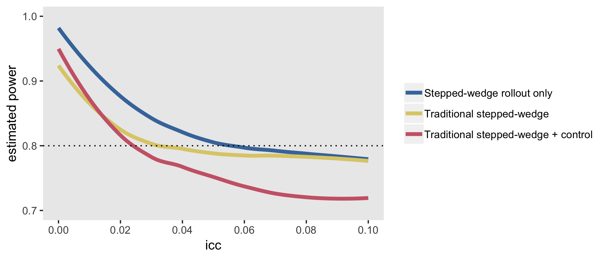
Thompson et al. provide more nuance that can improve power under different conditions - mostly involving changing period lengths or adding control-only sites, or both - but these simulations suggest that some sort of stepped-wedge design (either limited to the rollout phase or not) will generally be advantageous, at least under the strict requirements that I established to frame the design.
All of this has been done in the context of a normally distributed outcome. At some point, I will certainly re-do this comparison with a binary outcome.
Addendum: cluster randomized trial

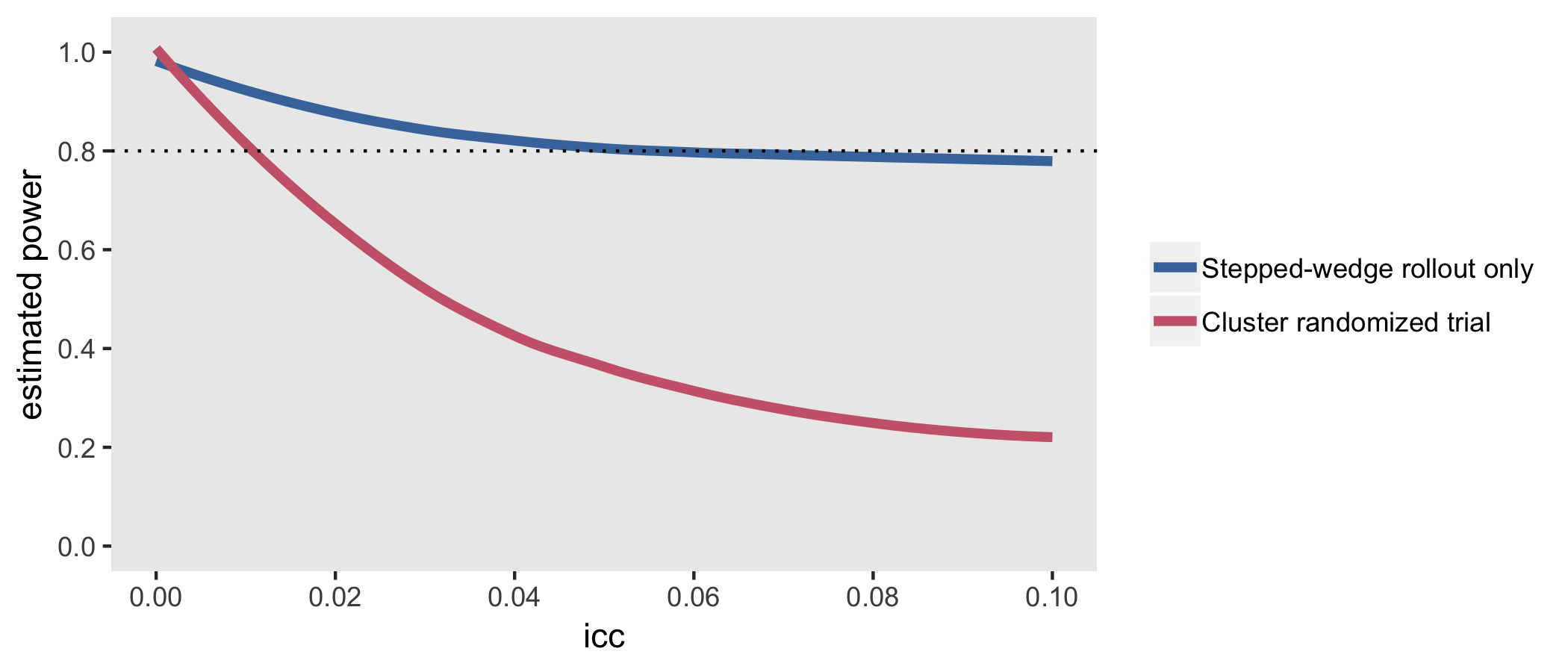
A traditional cluster randomized trial was not really under consideration because we declared that we could only deliver the intervention to 10 sites at any one time. However, it is illustrative to compare this design to make it clear that CRT is really best used when variability across sites is at its lowest (i.e. when the ICC is at or very close to zero). In this example, 25 sites are randomized to receive the intervention starting in the first week and 25 sites never receive the intervention. Data are collected for all 24 weeks for each of the 50 clusters.

The simulations confirm findings that the CRT is more efficient than stepped-wedge designs when the ICC is close to zero, but pales in comparison even with ICCs as low as 0.01:
