In the last post, I tried to provide a little insight into the chi-square test. In particular, I used simulation to demonstrate the relationship between the Poisson distribution of counts and the chi-squared distribution. The key point in that post was the role conditioning plays in that relationship by reducing variance.
To motivate some of the key issues, I talked a bit about recycling. I asked you to imagine a set of bins placed in different locations to collect glass bottles. I will stick with this scenario, but instead of just glass bottle bins, we now also have cardboard, plastic, and metal bins at each location. In this expanded scenario, we are interested in understanding the relationship between location and material. A key question that we might ask: is the distribution of materials the same across the sites? (Assume we are still just counting items and not considering volume or weight.)
Independence
If we tracked the number of items for a particular day, we could record the data in a contingency table, which in this case would be \(4 \times 3\) array. If we included the row and column totals, it might look like this:
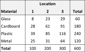
One way to inspect the data would be to calculate row- and column-specific proportions. From this (albeit stylized example), it is apparent that the proportion of each material is constant across locations - 10% of the items are glass, roughly 30% are cardboard, 40% are plastic, and 20% are metal. Likewise, for each material, about 17% are in location 1, 33% in location 2, and 50% in location 3:

This consistency in proportions across rows and columns is the hallmark of independence. In more formal terms, \(P(M = m | L = l) = P(M = m)\) and \(P(L = l|M = m) = P(L = l)\). The conditional probability (what we see in a particular row or column) is equal to the overall probability (what we see in the marginal (total) row or column.
The actual definition of statistical independence with respect to materials and location is
\[ P(M=m \ \& \ L= l) = P(M=m) \times P(L=l) \]
The probability on the left is the cell-specific proportion (the count of the number of items with \(M=m\) and \(L=l\) divided by \(N\), the total number of items in the entire table). The two terms on the right side of the equation are the marginal row and column probabilities respectively. The table of overall proportions gives us an example of data generated from two characteristics that are independent:
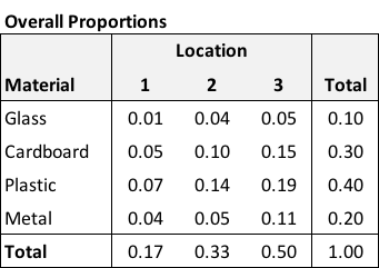
There are 116 plastic items in location 3, 19% of the overall items (\(116 \div 600\)). The overall proportion of plastic items is 40%, the overall proportion of items in location 3 is 50%, and \(0.19 \approx 0.4 \times 0.5\). If we inspect all of the cells, the same approximation will hold.
Dependence
In the case where the distributions of materials differ across locations, we no longer have independence. Here is an example, though note that the marginal totals are unchanged:
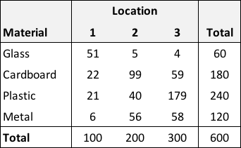
Looking across the row- and column-specific proportions, it is clear that something unique might be going on at each location:

It is apparent that the formal definition of independence might be violated: \(P(M=m \ \& \ L=l) \ne P(M=m)P(L=l\)). Look again at plastics in location 3: \(0.30 \ne 0.4 \times 0.5\).

The chi-square test of independence
I have been making declarations about independence with my made up contingency tables, just because I was the all-knowing creator who made them up. Of course, when we collect actual data, we don’t have that luxury. That is where the chi-square test of independence helps us.
Here’s the general idea. We start off by making the initial assumption that the rows and columns are indeed independent (this is actually our null hypothesis). We then define a test statistic \(X^2\) as
\[ X^2 = \sum_{m,l} \frac{(O_{ml} - E_{ml})^2}{E_{ml}}.\] This is just a slight modification of the test statistic we saw in part 1, which was presented as a summary of a \(k \times 1\) array. In this context, \(X^2\) is just a summary of the \(M \times \ L\) table. As previously discussed, \(X^2\) has a \(\chi^2\) distribution with a particular parameter specifying the \(k\) degrees freedom.
The question is, how can we calculate \(X^2\)? The observed data \(O_{ml}\) are just the observed data. But, we don’t necessarily know \(E_{ml}\), the expected value of each cell in the contingency table. These expected values can be defined as \(E_{ml} = P(M=m \ \& \ L=l) \times N\). If we assume that \(N\) is fixed, then we are half way there. All that remains is the joint probability of \(M\) and \(L\), \(P(M=m \ \& \ L=l)\). Under independence (which is our starting, or null, assumption) \(P(M=m \ \& \ L=l) = P(M=m)P(L=l)\). If we make the additional assumption that the row and column totals (margins) \(R_m\) and \(C_l\) are fixed, we can calculate \(P(M=m) = R_m/N\) and \(P(L=l) = C_l/N\). So now,
\[E_{ml} = \frac{(R_m * C_l)}{N}.\] Where does that leave us? We calculate the test statistic \(X^2\) and evaluate that statistic in the context of the theoretical sampling distribution suggested by the assumptions of independence and fixed marginal totals. That theoretical sampling distribution is \(\chi^2\) with some degrees of freedom. If the observed \(X^2\) is very large and defies the theoretical distribution (i.e. seems like an outlier), we will reject the notion of independence. (This is just null hypothesis testing using the \(X^2\) statistic.)
Chi-square tests of our two tables
The test statistic from the first table (which I suggest is from a scenario where material and location are independent) is relatively small. We would not conclude that material and location are associated:
##                 Sum
##       8  23  29  60
##      28  61  91 180
##      39  85 116 240
##      25  31  64 120
## Sum 100 200 300 600chisq.test(im)##
## Pearson's Chi-squared test
##
## data: im
## X-squared = 5.0569, df = 6, p-value = 0.5365In the second case, the test statistic \(X^2\) is quite large, leading us to conclude that material and location are indeed related, which is as we suspected:
##                 Sum
##      51   5   4  60
##      22  99  59 180
##      21  40 179 240
##       6  56  58 120
## Sum 100 200 300 600chisq.test(dm)##
## Pearson's Chi-squared test
##
## data: dm
## X-squared = 314.34, df = 6, p-value < 2.2e-16Degrees of freedom
The paramount question is what \(\chi^2\) distribution does \(X^2\) have under the independence assumption? If you look at the results of the chi-square tests above, you can see that, under the null hypothesis of independence and fixed margins, these tables have six degree of freedom, so \(X^2 \sim \chi^2_6\). But, how do we get there? What follows is a series of simulations that start with an unconditional data generation process and ends with the final set of marginal conditions. The idea is to show that by progressively adding stricter conditions to the assumptions, we continuously reduce variability and lower the degrees of freedom.
Unconditional contingency tables
If we start with a data generation process based on the \(4 \times 3\) table that has no conditions on the margins or total number of items, the statistic \(X^2\) is a function of 12 independent Poisson variables. Each cell has an expected value determined by row and column independence. It should follow that \(X^2\) will have 12 degrees of freedom. Simulating a large number of tables under these conditions and evaluating the distribution of the calculated \(X^2\) statistics will likely support this.
The initial (independent) table specified above is our starting point:
addmargins(im)## Sum
## 8 23 29 60
## 28 61 91 180
## 39 85 116 240
## 25 31 64 120
## Sum 100 200 300 600row <- margin.table(im, 1)
col <- margin.table(im, 2)
N <- sum(row)These are the expected values based on the observed row and column totals:
(expected <- (row/N) %*% t(col/N) * N)## [,1] [,2] [,3]
## [1,] 10 20 30
## [2,] 30 60 90
## [3,] 40 80 120
## [4,] 20 40 60Each randomly generated table is a collection of 12 independent Poisson random variables with \(\lambda_{ml}\) defined by the “expected” table. The tables are first generated as a collection columns and stored in a matrix. Here, I am creating 10,000 tables - and print out the first two in column form:
set.seed(2021)

(lambdas <-  as.vector(t(expected)))
## [1] 10 20 30 30 60 90 40 80 120 20 40 60condU <- matrix(rpois(n = 10000*length(lambdas),
lambda = lambdas),
nrow = length(lambdas))
condU[, 1:2]## [,1] [,2]
## [1,] 9 15
## [2,] 22 11
## [3,] 31 37
## [4,] 31 25
## [5,] 66 71
## [6,] 71 81
## [7,] 41 50
## [8,] 74 87
## [9,] 138 96
## [10,] 15 20
## [11,] 36 30
## [12,] 71 53Now, I convert each column to a table and create a “list” of tables. Here are the first two tables with the row and column margins; you can see that even the totals change from table to table:
condUm <- lapply(seq_len(ncol(condU)),
  function(i) matrix(condU[,i], length(row), length(col), byrow = T))

addmargins(condUm[[1]])
## Sum
## 9 22 31 62
## 31 66 71 168
## 41 74 138 253
## 15 36 71 122
## Sum 96 198 311 605addmargins(condUm[[2]])## Sum
## 15 11 37 63
## 25 71 81 177
## 50 87 96 233
## 20 30 53 103
## Sum 110 199 267 576A function avgMatrix estimates the average and variance of each of the cells (code can be made available if there is interest). The average of the 10,000 tables mirrors the “expected” table. And since all cells (including the totals) are Poisson distributed, the variance should be quite close to the mean table:
sumU <- avgMatrix(condUm, addMarg = T, sLabel = "U")

round(sumU$sampAvg, 0)
## [,1] [,2] [,3] [,4]
## [1,] 10 20 30 60
## [2,] 30 60 90 180
## [3,] 40 80 120 240
## [4,] 20 40 60 120
## [5,] 100 200 300 600round(sumU$sampVar, 0)## [,1] [,2] [,3] [,4]
## [1,] 10 19 30 60
## [2,] 30 61 90 180
## [3,] 40 80 124 244
## [4,] 20 40 60 122
## [5,] 100 199 308 613Function estX2 calculates the \(X^2\) statistic for each contingency table:
estX2 <- function(contMat, expMat) {
  X2 <- sum( (contMat - expMat)^2 / expMat)
  return(X2)
}

X2 <- sapply(condUm, function(x) estX2(x, expected))

head(X2)
## [1] 11.819444 23.162500 17.681944 3.569444 31.123611 14.836111Comparing the mean and variance of the 10,000 simulated \(X^2\) statistics with the mean and variance of data generated from a \(\chi^2_{12}\) distribution indicates that the two are quite close:
trueChisq <- rchisq(10000, 12)

# Comparing means
round(c( mean(X2), mean(trueChisq)), 1)
## [1] 12 12# Comparing variance
round(c( var(X2), var(trueChisq)), 1)## [1] 24.5 24.3Conditioning on N
If we assume that the total number of items remains the same from day to day (or sample to sample), but we allow to totals to vary by location and materials, we have a constrained contingency table that looks like this:
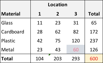
The table total is highlighted in yellow to indicate that \(N\) is fixed. The “metal/location 3” is also highlighted because once \(N\) is fixed and all the other cells are allowed to be randomly generated, that last cell is automatically determined as \[C_{metal, 3} = N - \sum_{ml \ne (metal \ \& \ 3)} C_{ml}.\] The data generation process that reflects this constraint is the multinomial distribution, which is the multivariate analogue to the binomial distribution. The cell probabilities are set based on the proportions of the independence table:
round(probs <- expected/N, 2)## [,1] [,2] [,3]
## [1,] 0.02 0.03 0.05
## [2,] 0.05 0.10 0.15
## [3,] 0.07 0.13 0.20
## [4,] 0.03 0.07 0.10As before with the unconditional scenario, let’s generate a large number of tables, each conditional on N. I’ll show two tables so you can see that N is indeed constrained:
condN <- rmultinom(n = 10000, size = N, prob = as.vector(t(probs)))
condNm <- lapply(seq_len(ncol(condN)),
                 function(i) matrix(condN[,i], length(row), length(col),
                                    byrow = T))
addmargins(condNm[[1]])
## Sum
## 12 16 30 58
## 26 67 83 176
## 36 91 119 246
## 21 40 59 120
## Sum 95 214 291 600addmargins(condNm[[2]])## Sum
## 8 20 19 47
## 30 64 97 191
## 36 84 112 232
## 21 52 57 130
## Sum 95 220 285 600And here is the key point: if we look at the mean of the cell counts across the samples, they mirror the expected values. But, the variances are slightly reduced. We are essentially looking at a subset of the samples generated above that were completely unconstrained, and in this subset the total across all cells equals \(N\). As I demonstrated in the last post, this constraint effectively removes samples with more extreme values in some of the cells - which reduces the variance of each cell:
sumN <- avgMatrix(condNm, sLabel = "N")

round(sumN$sampAvg, 0)
## [,1] [,2] [,3]
## [1,] 10 20 30
## [2,] 30 60 90
## [3,] 40 80 120
## [4,] 20 40 60round(sumN$sampVar, 0)## [,1] [,2] [,3]
## [1,] 10 19 29
## [2,] 28 53 76
## [3,] 37 70 95
## [4,] 19 39 54We lost one degree of freedom (the one cell highlighted in grey in the table above), so it makes sense to compare the distribution of \(X^2\) to a \(\chi^2_{11}\):
X2 <- sapply(condNm, function(x) estX2(x, expected))

trueChisq <- rchisq(10000, 11)

# Comparing means
round(c( mean(X2), mean(trueChisq)), 1)
## [1] 11 11# Comparing variance
round(c( var(X2), var(trueChisq)), 1)## [1] 21.7 22.4Conditioning on row totals
We go one step further - and condition on the row totals (I am going to skip conditioning on the column totals, because conceptually it is the same thing). Now, the row totals in the table are highlighted, and all of the cells in “location 3” are grayed out. Once the row total is set, and the first two elements in each row are generated, the last cell in the row is determined. We are losing four degrees of freedom.
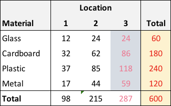
These tables can be generated again using the multinomial distribution, but each row of the table is generated individually. The cell probabilities are all based on the overall column proportions:
round(prob <- col/N, 2)## [1] 0.17 0.33 0.50The rows are generated individually based on the count of the total number fixed items in the row. Two of the tables are shown again to show that the generated tables have the same row totals:
condRow <- lapply(seq_len(length(row)),
              function(i) t(rmultinom(10000, size = row[i],prob=prob)))

condRm <- lapply(seq_len(10000),
              function(i) {
                  do.call(rbind, lapply(condRow, function(x) x[i,]))
              }
)

addmargins(condRm[[1]])
## Sum
## 5 19 36 60
## 32 55 93 180
## 39 76 125 240
## 19 42 59 120
## Sum 95 192 313 600addmargins(condRm[[2]])## Sum
## 11 19 30 60
## 36 52 92 180
## 44 74 122 240
## 16 41 63 120
## Sum 107 186 307 600This time around, the variance of the cells is reduced even further:
sumR <- avgMatrix(condRm, sLabel = "R")

round(sumR$sampAvg, 0)
## [,1] [,2] [,3]
## [1,] 10 20 30
## [2,] 30 60 90
## [3,] 40 80 120
## [4,] 20 40 60round(sumR$sampVar, 0)## [,1] [,2] [,3]
## [1,] 8 14 15
## [2,] 26 41 46
## [3,] 34 53 59
## [4,] 17 27 31And let’s compare the distribution of the sample \(X^2\) statistics with the \(\chi^2_8\) distribution (since we now have \(12 - 4 = 8\) degrees of freedom):
X2 <- sapply(condRm, function(x) estX2(x, expected))

trueChisq <- rchisq(10000, 8)

# Comparing means
round(c( mean(X2), mean(trueChisq)), 1)
## [1] 8.1 8.0# Comparing variance
round(c( var(X2), var(trueChisq)), 1)## [1] 16.4 16.4Conditioning on both row and column totals
Here we are at the grand finale, the actual chi-square test of independence, where we condition on both the row and column totals. The whole point of this is to show that once we set this condition, the variance of the cells is reduced far below the Poisson variance. As a result, we must use a \(\chi^2\) distribution with fewer degrees of freedom when evaluating the \(X^2\) test statistic.
This final table shows both the constraints on the row and column totals, and the impact on the specific cell. The six grayed out cells are determined by the column totals once the six other cells are generated. That is, we lose six degrees of freedom. (Maybe you can now see where the \(degrees \ of \ freedom = (\# \ rows - 1) \times (\# \ cols - 1)\) comes from?)
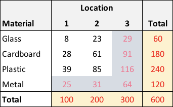
The process for generating data for a table where both row totals and column totals is interesting, and I actually wrote some pretty inefficient code that was based on a simple algorithm tied to the multivariate hypergeometric distribution, which was described here. Luckily, just as I started writing this section, I stumbled upon the R function r2dtable. (Not sure why I didn’t find it right away, but was glad to have found it in any case.) So, with a single line, 10,000 tables can be very quickly generated.
condRCm <- r2dtable(10000, row, col)Here are the first two generated tables:
addmargins(condRCm[[1]])## Sum
## 14 12 34 60
## 24 64 92 180
## 38 79 123 240
## 24 45 51 120
## Sum 100 200 300 600addmargins(condRCm[[2]])## Sum
## 7 23 30 60
## 30 60 90 180
## 38 78 124 240
## 25 39 56 120
## Sum 100 200 300 600And with this most restrictive set of conditioning constraints, the variances of the cell counts are considerably lower than when conditioning on row or column totals alone:
sumRC <- avgMatrix(condRCm, sLabel = "RC")

round(sumRC$sampAvg, 0)
## [,1] [,2] [,3]
## [1,] 10 20 30
## [2,] 30 60 90
## [3,] 40 80 120
## [4,] 20 40 60round(sumRC$sampVar, 0)## [,1] [,2] [,3]
## [1,] 8 12 13
## [2,] 18 28 31
## [3,] 20 32 36
## [4,] 13 22 24And, take a look at the mean and variance of the \(X^2\) statistic as it compares to the mean and variance of the \(\chi^2_6\) distribution:
X2 <- sapply(condRCm, function(x) estX2(x, expected))

trueChisq <- rchisq(10000, 6)

# Comparing means
round(c( mean(X2), mean(trueChisq)), 1)
## [1] 6 6# Comparing variance
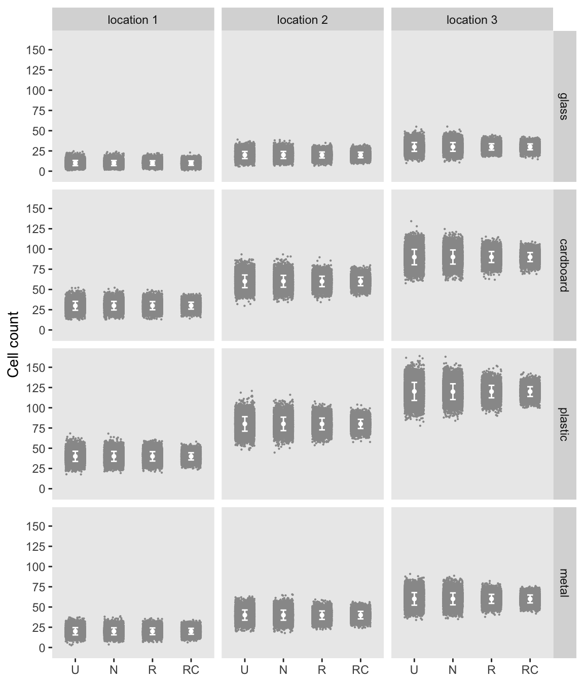
round(c( var(X2), var(trueChisq)), 1)## [1] 11.8 11.7I’ll leave you with a plot of the cell counts for each of the 10,000 tables generated in each of the conditioning scenarios: unconditional (U), conditional on N (N), conditional on row totals (R), and conditional on both row and column totals (RC). This plot confirms the point I’ve been trying to make in this post and the last: adding more and more restrictive conditions progessively reduces variability within each cell. The reduction in degrees of freedom in the chi-square test is the direct consequence of this reduction in within-cell variability.
