Kids today are so sophisticated (at least they are in New York City, where I live). While I didn’t hear about the chi-square test of independence until my first stint in graduate school, they’re already talking about it in high school. When my kids came home and started talking about it, I did what I usually do when they come home asking about a new statistical concept. I opened up R and started generating some data. Of course, they rolled their eyes, but when the evening was done, I had something that might illuminate some of what underlies the theory of this ubiquitous test.
Actually, I created enough simulations to justify two posts - so this is just part 1, focusing on the distribution and its relationship to the Poisson distribution. Part 2 will consider contingency tables, where we are often interested in understanding the nature of the relationship between two categorical variables. More on that the next time.
The chi-square distribution
The chi-square (or ) distribution can be described in many ways (for example as a special case of the Gamma distribution), but it is most intuitively characterized in relation to the standard normal distribution, . The distribution has a single parameter which represents the degrees of freedom. If is standard normal, (i.e ), then has a distribution. If is also standard normal, then . That is, if we add two squared standard normal random variables, the distribution of the sum is chi-squared with 2 degrees of freedom. More generally,
where each .
The following code defines a data set with two standard normal random variables and their sum:
library(simstudy)

def <- defData(varname = "x", formula = 0, variance = 1, dist = "normal")
def <- defData(def, "chisq1df", formula = "x^2", dist = "nonrandom")
def <- defData(def, "y", formula = 0, variance = 1, dist = "normal")
def <- defData(def, "chisq2df",
               formula = "(x^2) + (y^2)", dist = "nonrandom")

set.seed(2018)
dt <- genData(10000, def)

dt[1:5,]
## id x chisq1df y chisq2df
## 1: 1 -0.42298398 0.178915450 0.05378131 0.181807879
## 2: 2 -1.54987816 2.402122316 0.70312385 2.896505464
## 3: 3 -0.06442932 0.004151137 -0.07412058 0.009644997
## 4: 4 0.27088135 0.073376707 -1.09181873 1.265444851
## 5: 5 1.73528367 3.011209400 -0.79937643 3.650212075The standard normal has mean zero and variance one. Approximately 95% of the values will be expected to fall within two standard deviations of zero. Here is your classic “bell” curve:
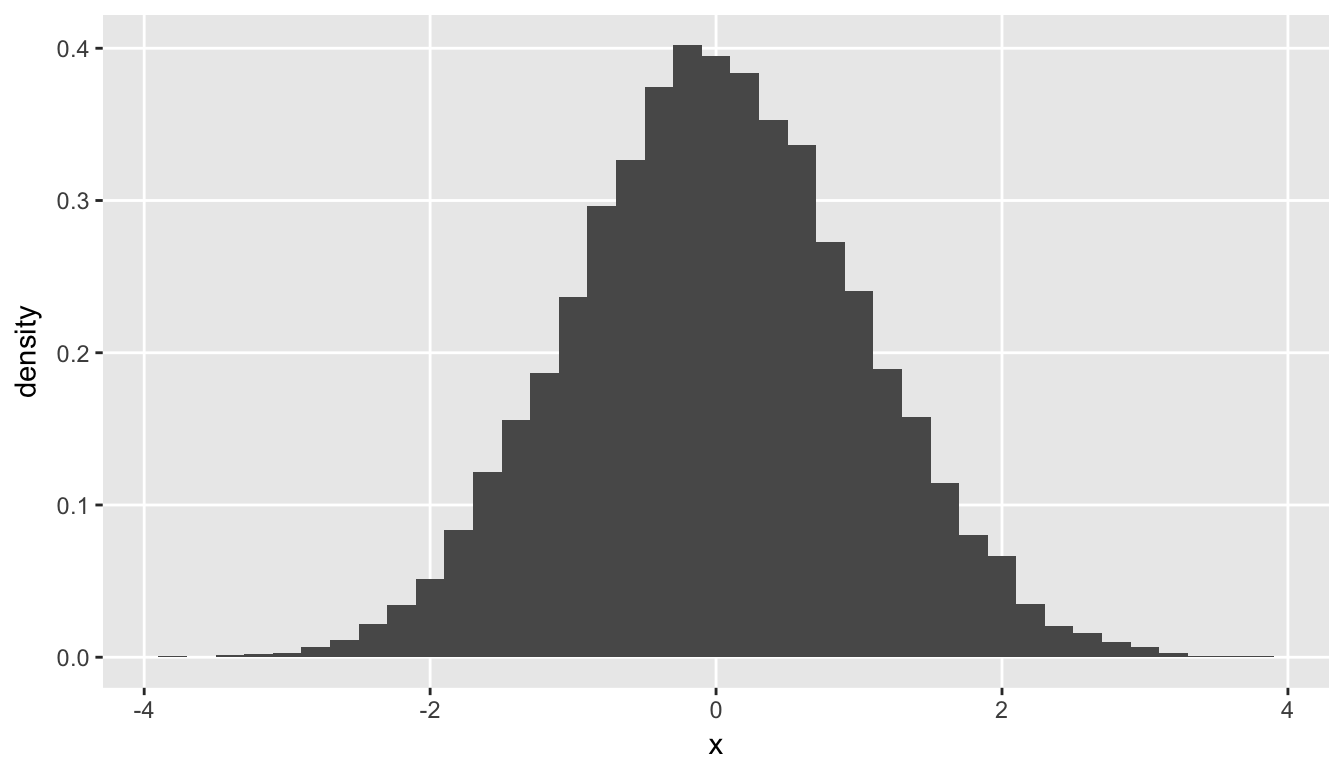
Since the statistic (try not to confuse and , unfortunate I know) is the sum of the squares of a continuous random variable and is always greater or equal to zero, the is a distribution of positive, continuous measures. Here is a histogram of chisq1df from the data set dt, which has a distribution:
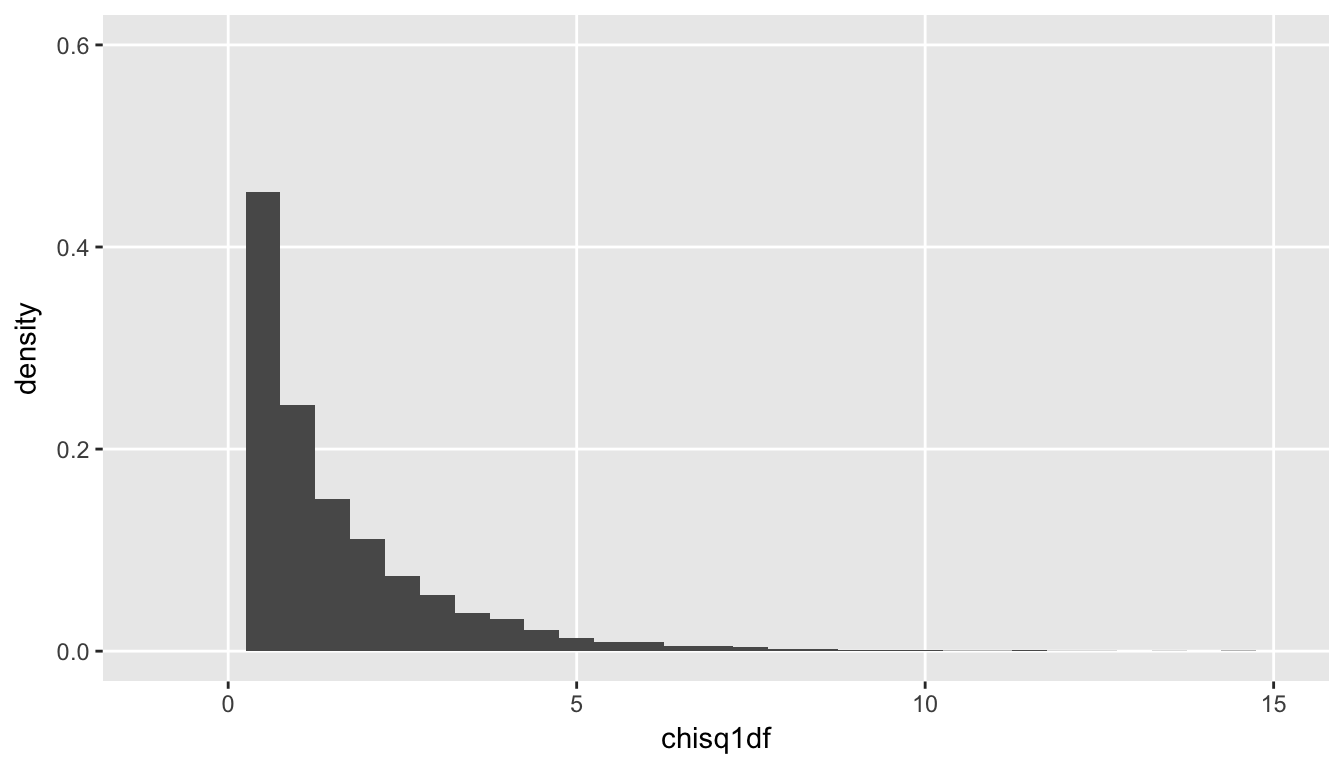
And here is a plot of chisq2df, which has two degrees of freedom, and has a distribution. Unsurprisingly, since we are adding positive numbers, we start to see values further away from zero:
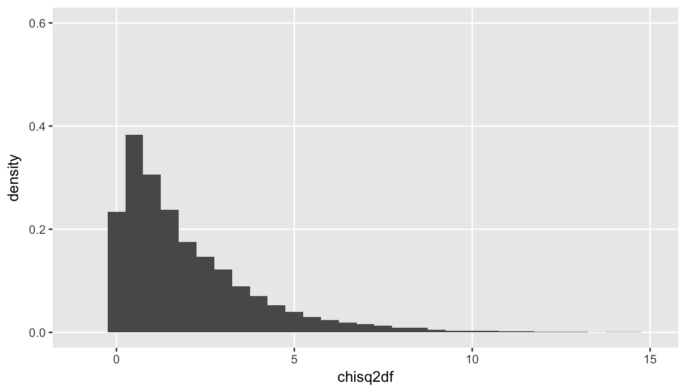
Just to show that the data we generated by adding two squared standard normal random variables is actually distributed as a , we can generate data from this distribution directly, and overlay the plots:
actual_chisq2 <- rchisq(10000, 2)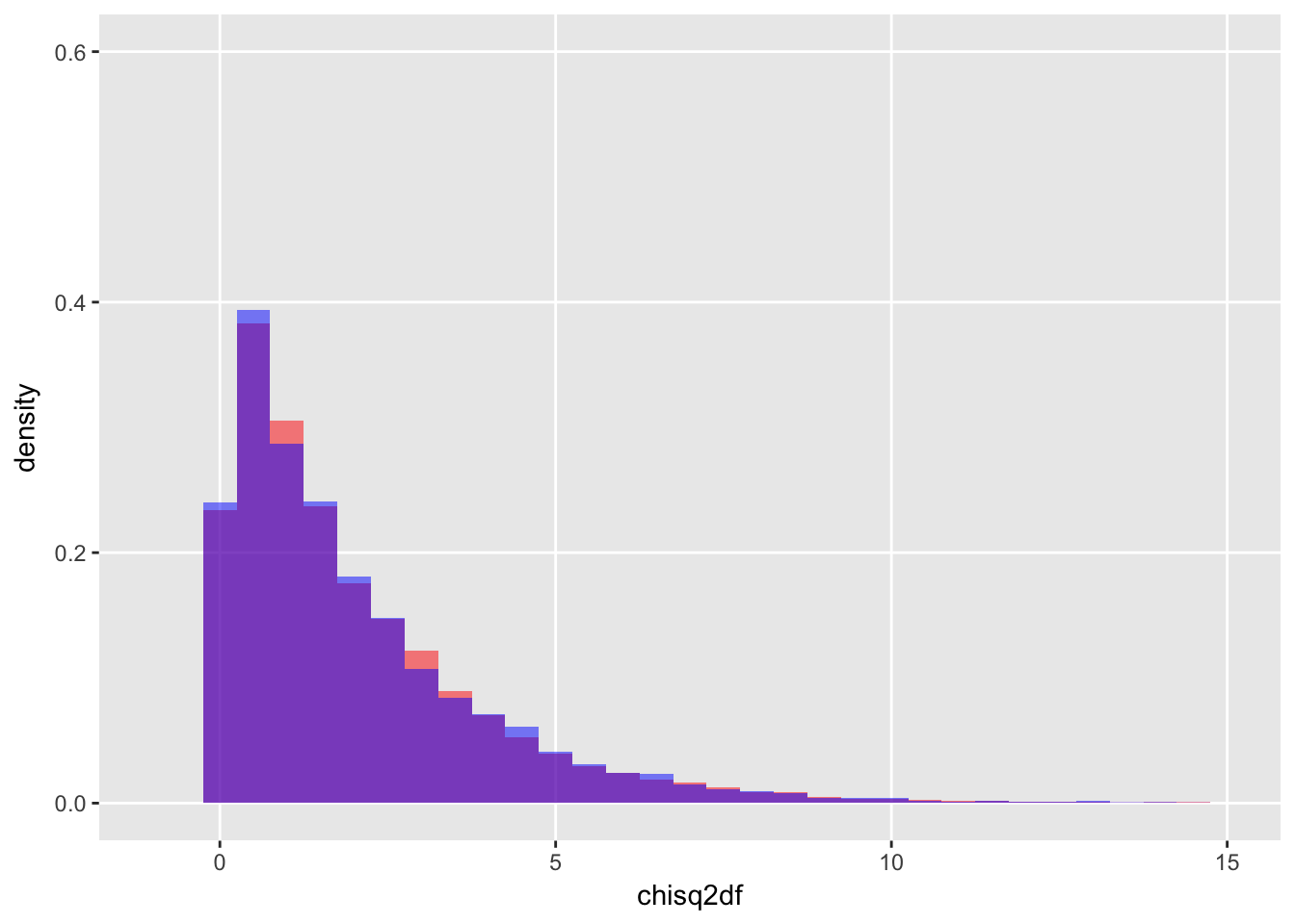
Recycling and the Poisson distribution
When we talk about counts, we are often dealing with a Poisson distribution. An example I use below is the number of glass bottles that end up in an apartment building’s recycling bin every day (as I mentioned, I do live in New York City). The Poisson distribution is a non-negative, discrete distribution that is characterized by a single parameter . If , then .
def <- defData(varname = "h", formula = 40, dist = "poisson")

dh <- genData(10000, def)

round(dh[, .(avg = mean(h), var = var(h))], 1)
## avg var
## 1: 40.1 40To standardize a normally distributed variable (such as ), we subtract the mean and divide by the standard deviation:
and . Analogously, to standardize a Poisson variable we do the same, since is the mean and the variance:
The distribution of this standardized variable will be close to a standard normal. We can generate some data and check this out. In this case, the mean and variance of the Poisson variable is 40:
defA <- defDataAdd(varname = "s", formula = "(h-40)/sqrt(40)",
               dist = "nonrandom")

dh <- addColumns(defA, dh)
dh[1:5, ]
## id h s
## 1: 1 34 -0.9486833
## 2: 2 44 0.6324555
## 3: 3 37 -0.4743416
## 4: 4 46 0.9486833
## 5: 5 42 0.3162278The mean and variance of the standardized data do suggest a standardized normal distribution:
round(dh[ , .(mean = mean(s), var = var(s))], 1)## mean var
## 1: 0 1Overlaying the plots of the standardized poisson distribution with the standard normal distribution, we can see that they are quite similar:
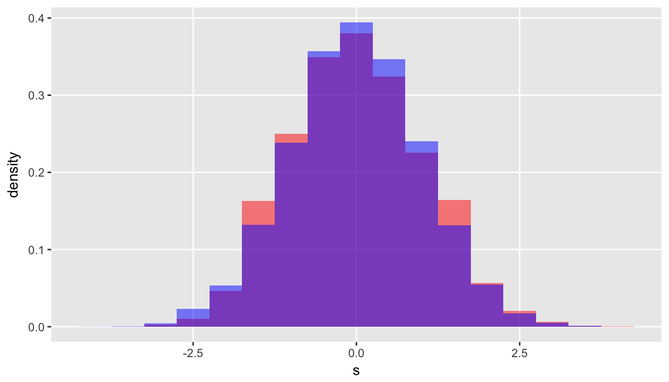
Since the standardized Poisson is roughly standard normal, the square of the standardized Poisson should be roughly . If we square normalized Poisson, this is what we have:
Or maybe in a more familiar form (think Pearson):
where is the observed value and is the expected value. Since is the expected value (and variance) of the Poisson random variable, the two formulations are equivalent.
Adding the transformed data to the data set, and calculating the mean and variance, it is apparent that these observations are close to a distribution:
defA <- defDataAdd(varname = "h.chisq", formula = "(h-40)^2/40",
               dist = "nonrandom")

dh <- addColumns(defA, dh)

round(dh[, .(avg = mean(h.chisq), var = var(h.chisq))], 2)
## avg var
## 1: 1 1.97actual_chisq1 <- rchisq(10000, 1)
round(c(avg = mean(actual_chisq1), var = var(actual_chisq1)), 2)## avg var
## 0.99 2.04Once again, an overlay of the two distributions based on the data we generated shows that this is plausible:
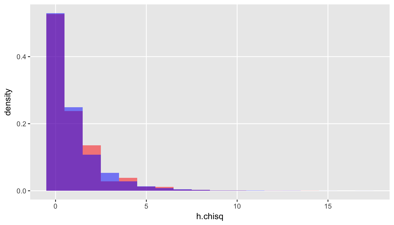
Just for fun, let’s repeatedly generate 10 Poisson variables each with its own value of and calculate for each iteration to compare with data generated from a distribution:
nObs <- 10000
nMeasures <- 10

lambdas <- rpois(nMeasures, 50)
poisMat <- matrix(rpois(n = nMeasures*nObs, lambda = lambdas),
                  ncol = nMeasures, byrow = T)

poisMat[1:5,]
## [,1] [,2] [,3] [,4] [,5] [,6] [,7] [,8] [,9] [,10]
## [1,] 48 51 49 61 59 51 67 35 43 39
## [2,] 32 58 49 67 57 35 69 40 57 55
## [3,] 44 50 60 56 57 49 68 49 48 32
## [4,] 44 44 42 49 52 50 63 39 51 38
## [5,] 42 38 62 57 62 40 68 34 41 58Each column (variable) has its own mean and variance:
rbind(lambdas,
      mean = apply(poisMat, 2, function(x) round(mean(x), 0)),
      var = apply(poisMat, 2, function(x) round(var(x), 0))
)
## [,1] [,2] [,3] [,4] [,5] [,6] [,7] [,8] [,9] [,10]
## lambdas 43 45 51 61 55 46 62 35 48 47
## mean 43 45 51 61 55 46 62 35 48 47
## var 43 46 51 61 55 46 62 35 47 47Calculate for each iteration (i.e. each row of the matrix poisMat), and estimate mean and variance across all estimated values of :
X2 <- sapply(seq_len(nObs),
             function(x) sum((poisMat[x,] - lambdas)^2 / lambdas))

round(c(mean(X2), var(X2)), 1)
## [1] 10.0 20.2The true distribution with 10 degrees of freedom:
chisqkdf <- rchisq(nObs, nMeasures)
round(c(mean(chisqkdf), var(chisqkdf)), 1)
## [1] 10.0 19.8These simulations strongly suggest that summing across independent standardized Poisson variables generates a statistic that has a distribution.
The consequences of conditioning
If we find ourselves in the situation where we have some number of bins or containers or cells into which we are throwing a fixed number of something, we are no longer in the realm of independent, unconditional Poisson random variables. This has implications for our statistic.
As an example, say we have those recycling bins again (this time five) and a total of 100 glass bottles. If each bottle has an equal chance of ending up in any of the five bins, we would expect on average 20 bottles to end up in each. Typically, we highlight the fact that under this constraint (of having 100 bottles) information about about four of the bins is the same as having information about all five. If I tell you that the first four bins contain a total of 84 bottles, we know that the last bin must have exactly 16. Actually counting those bottles in the fifth bin provides no additional information. In this case (where we really only have 4 pieces of information, and not the the 5 we are looking at), we say we have lost 1 degree of freedom due to the constraint. This loss gets translated into the chi-square test.
I want to explore more concretely how the constraint on the total number of bottles affects the distribution of the statistic and ultimately the chi-square test.
Unconditional counting
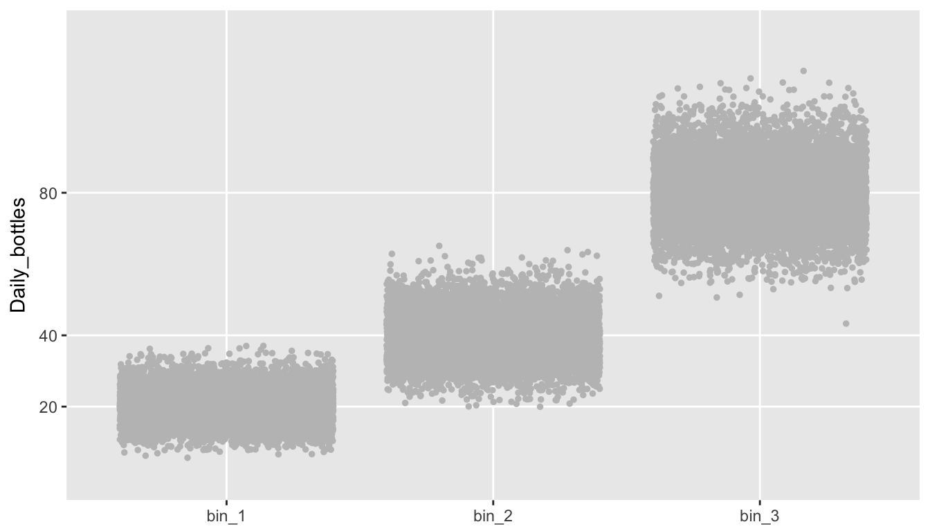
Consider a simpler example of three glass recycling bins in three different buildings. We know that, on average, the bin in building 1 typically has 20 bottles deposited daily, the bin in building 2 usually has 40, and the bin in building 3 has 80. These number of bottles in each bin is Poisson distributed, with equal to 20, 40, and 80, respectively. Note, while we would expect on average 140 total bottles across the three buildings, some days we have fewer, some days we have more - all depending on what happens in each individual building. The total is also Poisson distributed with .
Let’s generate 10,000 days worth of data (under the assumption that bottle disposal patterns are consistent over a very long time, a dubious assumption).
library(simstudy)

def <- defData(varname = "bin_1", formula = 20, dist = "poisson")
def <- defData(def, "bin_2", formula = 40, dist = "poisson")
def <- defData(def, "bin_3", formula = 80, dist = "poisson")
def <- defData(def, varname = "N",
               formula = "bin_1 + bin_2 + bin_3",
               dist = "nonrandom")


set.seed(1234)
dt <- genData(10000, def)

dt[1:5, ]
## id bin_1 bin_2 bin_3 N
## 1: 1 14 44 59 117
## 2: 2 21 36 81 138
## 3: 3 21 34 68 123
## 4: 4 16 43 81 140
## 5: 5 22 44 86 152The means and variances are as expected:
round(dt[ ,.(mean(bin_1), mean(bin_2), mean(bin_3))], 1)## V1 V2 V3
## 1: 20 39.9 80.1round(dt[ ,.(var(bin_1), var(bin_2), var(bin_3))], 1)## V1 V2 V3
## 1: 19.7 39.7 80.6This plot shows the actual numbers of bottles in each bin in each building over the 10,000 days:
There is also quite a lot of variability in the daily totals calculated by adding up the bins across three buildings. (While it is clear based on the mean and variance that this total has a distribution, the plot looks quite symmetrical. It is the case that as increases, the Poisson distribution becomes well approximated by the normal distribution.)
round(dt[, .(avgN = mean(N), varN = var(N))], 1)## avgN varN
## 1: 140 139.6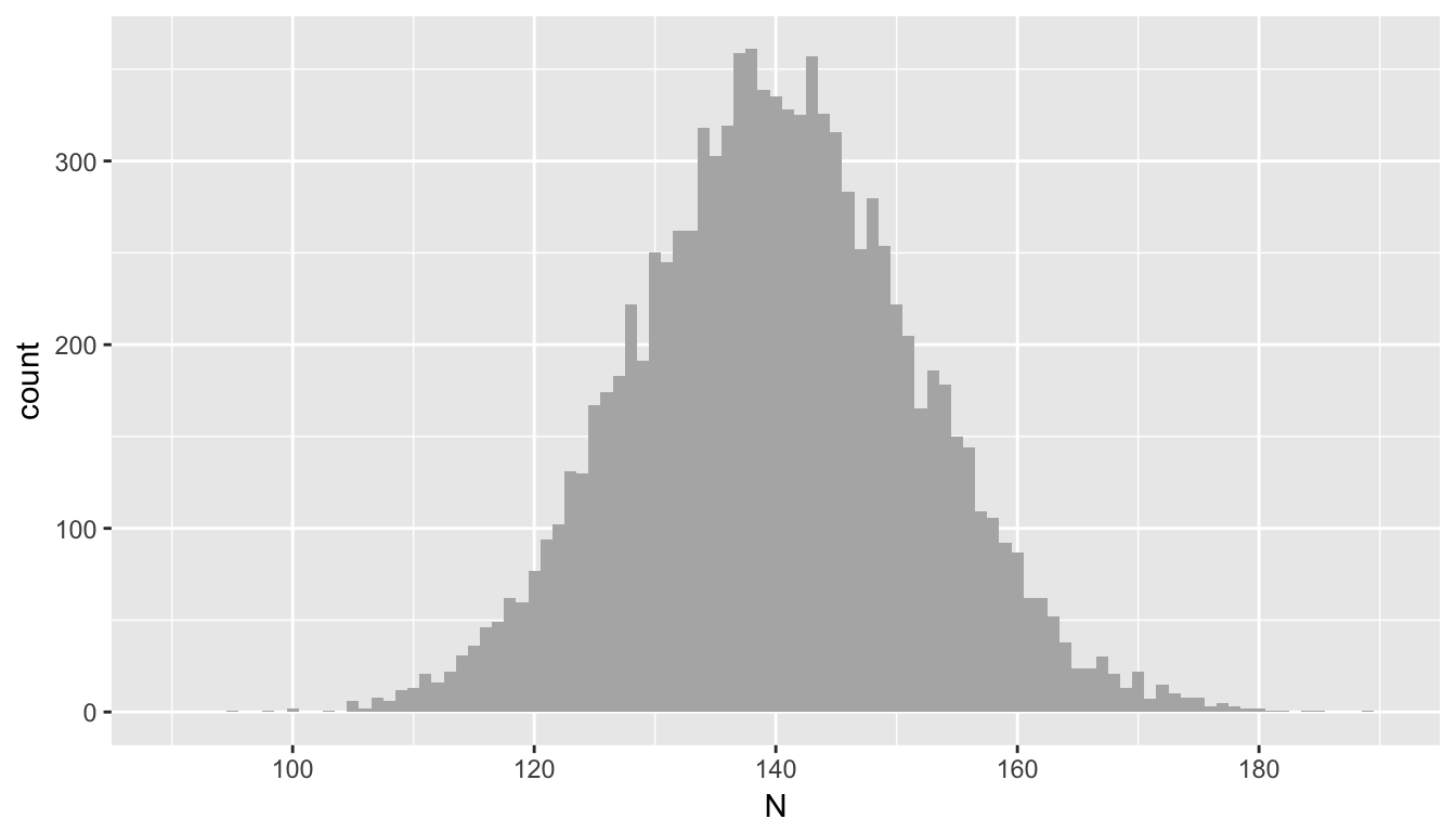
Conditional counting
Now, let’s say that the three bins are actually in the same (very large) building, located in different rooms in the basement, just to make it more convenient for residents (in case you are wondering, my bins are right next to the service elevator). But, let’s also make the assumption (and condition) that there are always between 138 and 142 total bottles on any given day. The expected values for each bin remain 20, 40, and 80, respectively.
We calculate the total number of bottles every day and identify all cases where the sum of the three bins is within the fixed range. For this subset of the sample, we see that the means are unchanged:
defAdd <- defDataAdd(varname = "condN",
                     formula = "(N >= 138 & N <= 142)",
                     dist = "nonrandom")

dt <- addColumns(defAdd, dt)

round(dt[condN == 1,
         .(mean(bin_1), mean(bin_2), mean(bin_3))],
      1)
## V1 V2 V3
## 1: 20.1 40 79.9However, and this is really the key point, the variance of the sample (which is conditional on the sum being between 138 and 142) is reduced:
round(dt[condN == 1,
         .(var(bin_1), var(bin_2), var(bin_3))],
      1)
## V1 V2 V3
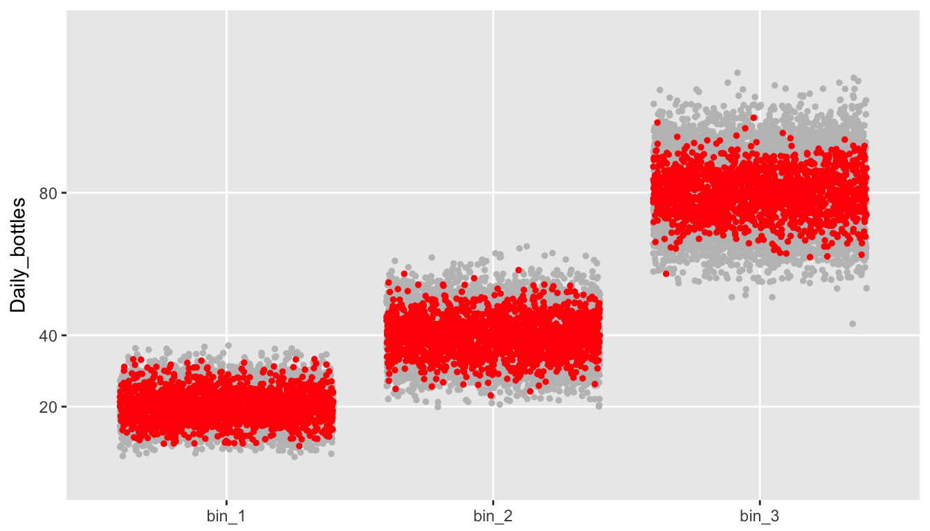
## 1: 17.2 28.3 35.4The red points in the plot below represent all daily totals that fall between 138 and 142 bottles. The spread from top to bottom is contained by the rest of the (unconstrained) sample, an indication that the variance for this conditional scenario is smaller:
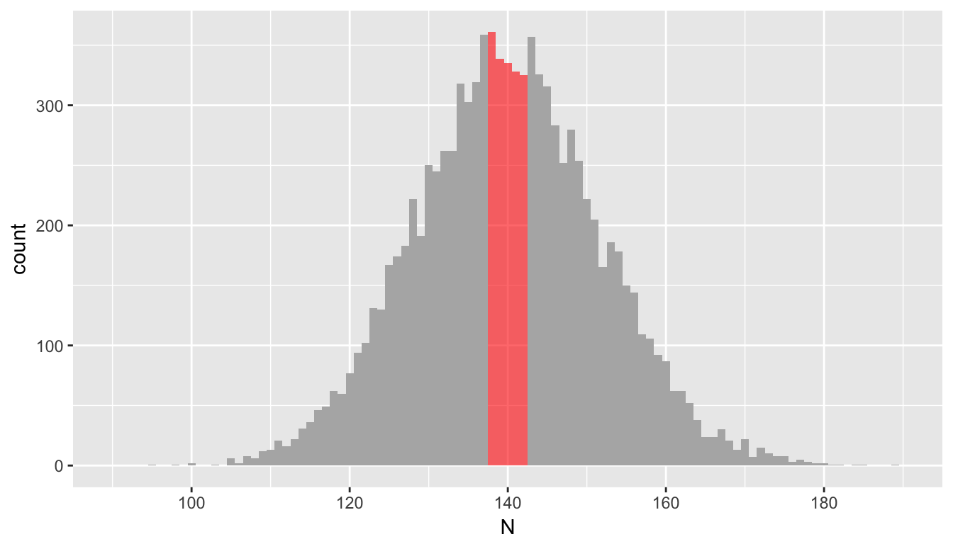
Not surprisingly, the distribution of the totals across the bins is quite narrow. But, this is almost a tautology, since this is how we defined the sample:
Biased standardization
And here is the grand finale of part 1. When we calculate using the standard formula under a constrained data generating process, we are not dividing by the proper variance. We just saw that the conditional variance within each bin is smaller than the variance of the unconstrained Poisson distribution. So, , as defined by
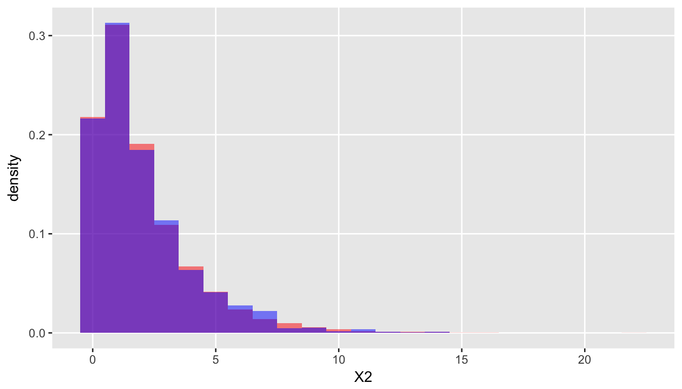
is not a sum of approximately standard normal variables - the variance used in the formula is too high. will be smaller than a . How much smaller? Well, if the constraint is even tighter, limited to where the total equals exactly 140 bottles every day, has a distribution.
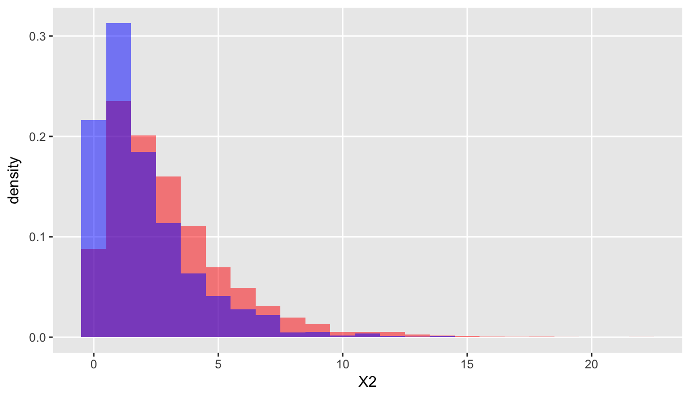
Even using our slightly looser constraint of fixing the total between 138 and 142, the distribution is quite close to a distribution:
defA <- defDataAdd(varname = "X2.1",
                   formula = "(bin_1-20)^2 / 20", dist = "nonrandom")
defA <- defDataAdd(defA, "X2.2",
                   formula = "(bin_2-40)^2 / 40", dist = "nonrandom")
defA <- defDataAdd(defA, "X2.3",
                   formula = "(bin_3-80)^2 / 80", dist = "nonrandom")
defA <- defDataAdd(defA, "X2",
                   formula = "X2.1 + X2.2 + X2.3", dist = "nonrandom")

dt <- addColumns(defA, dt)
Comparison with shows clear bias:
Here it is with a distribution:
Recycling more than glass
Part 2 will extend this discussion to the contingency table, which is essentially a 2-dimensional array of bins. If we have different types of materials to recycle - glass bottles, plastic containers, cardboard boxes, and metal cans - we need four bins at each location. We might be interested in knowing if the distribution of these four materials is different across the 3 different locations - this is where the chi-square test for independence can be useful.
As an added bonus, you can expect to see lots of code that allows you to simulate contingency tables under different assumptions of conditioning. I know my kids are psyched.