I’ve never taught an intro probability/statistics course. If I ever did, I would certainly want to bring the underlying wonder of the subject to life. I’ve always found it almost magical the way mathematical formulation can be mirrored by computer simulation, the way proof can be guided by observed data generation processes, and the way DGPs can confirm analytic solutions.
I would like to begin such a course with a somewhat unusual but accessible problem that would evoke these themes from the start. The concepts would not necessarily be immediately comprehensible, but rather would pique the interest of the students.
I recently picked up copy of John Allen Paulos’ fun sort-of-memoir A Numerate Life, and he reminded me of an interesting problem that might provide a good starting point for my imaginary course. The problem is great, because it is easy to understand, but challenging enough to raise some interesting issues. In this post, I sketch out a set of simulations and mathematical derivations that would motivate the ideas of marginal and conditional probability distributions.
The problem
Say we make repeated draws of independent uniform variables between 0 and 1, and add them up as we go along. The question is, on average, how many draws do we need to make so that the cumulative sum is greater than 1? We definitely need to make at least 2 draws, but it is possible (though almost certainly not the case) that we won’t get to 1 with even 100 draws. It turns that if we did this experiment over and over, the average number of draws would approach . Can we prove this and confirm by simulation?
Re-formulating the question more formally
If is one draw of a uniform random variable (where ), and represents the number of draws, the probability of taking on a specific value (say ) can be characterized like this:
Now, we need to understand this a little better to figure out how to figure out how to characterize the distribution of , which is what we are really interested in.
CDF
This is where I would start to describe the concept of a probability distribution, and start by looking at the cumulative distribution function (CDF) for a fixed . It turns out that the CDF for this distribution (which actually has at least two names - Irwin-Hall distribution or uniform sum distribution) can be estimated with the following equation. (I certainly wouldn’t be bold enough to attempt to derive this formula in an introductory class):
Our first simulation would confirm that this specification of the CDF is correct. Before doing the simulation, we create an R function to calculate the theoretical cumulative probability for the range of .
psumunif <- function(x, n) {

  k <- c(0:floor(x))
  (1/factorial(n)) * sum( (-1)^k * choose(n, k) * (x - k)^n )

}

ddtheory <- data.table(x = seq(0, 3, by = .1))
ddtheory[, cump := psumunif(x, 3), keyby = x]

ddtheory[x %in% seq(0, 3, by = .5)]
## x cump
## 1: 0.0 0.000
## 2: 0.5 0.021
## 3: 1.0 0.167
## 4: 1.5 0.500
## 5: 2.0 0.833
## 6: 2.5 0.979
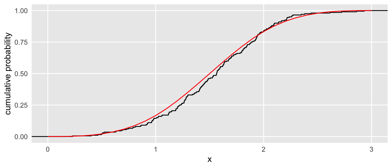
## 7: 3.0 1.000Now, we generate some actual data. In this case, we are assuming three draws for each experiment, and we are “conducting” 200 different experiments. We generate non-correlated uniform data for each experiment:
library(simstudy)
set.seed(02012019)

dd <- genCorGen(n = 200, nvars = 3, params1 = 0, params2 = 1,
          dist = "uniform", rho = 0.0, corstr = "cs", cnames = "u")
dd
## id period u
## 1: 1 0 0.98
## 2: 1 1 0.44
## 3: 1 2 0.58
## 4: 2 0 0.93
## 5: 2 1 0.80
## ---
## 596: 199 1 0.44
## 597: 199 2 0.77
## 598: 200 0 0.21
## 599: 200 1 0.45
## 600: 200 2 0.83For each experiment, we calculate the sum the of the three draws, so that we have a data set with 200 observations:
dsum <- dd[, .(x = sum(u)), keyby = id]
dsum
## id x
## 1: 1 2.0
## 2: 2 1.8
## 3: 3 1.6
## 4: 4 1.4
## 5: 5 1.6
## ---
## 196: 196 1.7
## 197: 197 1.3
## 198: 198 1.4
## 199: 199 1.7
## 200: 200 1.5We can plot the theoretical CDF versus the observed empirical CDF:
ggplot(dsum, aes(x)) +
  stat_ecdf(geom = "step", color = "black") +
  geom_line(data=ddtheory, aes(x=x, y = cump), color ="red") +
  scale_x_continuous(limits = c(0, 3)) +
  ylab("cumulative probability") +
  theme(panel.grid.minor = element_blank(),
        axis.ticks = element_blank())
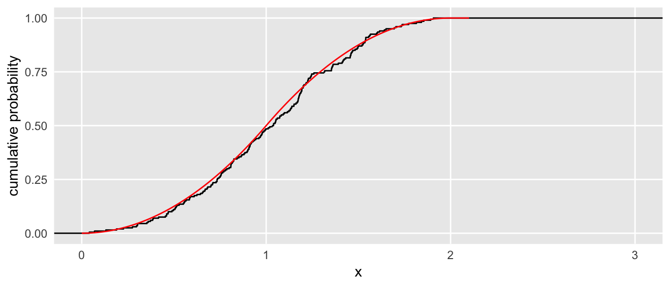
And here is another pair of curves using a set of experiments with only two draws for each experiment:

More specifically, exploring P(sum < 1)
The problem at hand specifically asks us to evaluate . So this will be our first algebraic manipulation to derive the probability in terms of , starting with the analytic solution for the CDF I introduced above without derivation:
We can look back at the plots to confirm that this solution is matched by the theoretical and empirical CDFs. For , we expect . And for , the expected probability is .
Deriving
I think until this point, things would be generally pretty accessible to a group of students thinking about these things for the first time. This next step, deriving might present more of a challenge, because we have to deal with joint probabilities as well as conditional probabilities. While I don’t do so here, I think in a classroom setting I would delve more into the simulated data to illustrate each type of probability. The joint probability is merely a probability of multiple events occurring simultaneously. And the the conditional probability is a probability of an event for a subset of the data (the subset defined by the group of observations where another - conditional - event actually happened). Once those concepts were explained a bit, I would need a little courage to walk through the derivation. However, I think it would be worth it, because moving through each step highlights an important concept.
is a new random variable that takes on the value if and . That is, the value in a sequence uniform random variables is the threshold where the cumulative sum exceeds 1. can be derived as follows:
Now, once we get to this point, it is just algebraic manipulation to get to the final formulation. It is a pet peeve of mine when papers say that it is quite easily shown that some formula can be simplified into another without showing it; sometimes, it is not so simple. In this case, however, I actually think it is. So, here is a final solution of the probability:
Simulating the distribution of
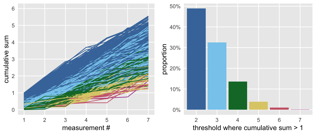
We are almost there. To simulate , we generate 1000 iterations of 7 draws. For each iteration, we check to see which draw pushes the cumulative sum over 1, and this is the observed value of for each iteration. Even though can conceivably be quite large, we stop at 7, since the probability of observing is vanishingly small, .
dd <- genCorGen(n = 1000, nvars = 7, params1 = 0, params2 = 1,
          dist = "uniform", rho = 0.0, corstr = "cs", cnames = "U")

dd[, csum := cumsum(U), keyby = id]
dd[, under := 1*(csum < 1)]

dc <- dcast(dd, id ~ (period + 1), value.var = c("under", "csum" ))
dc[, n := 2 + sum(under_2, under_3, under_4, under_5, under_6, under_7),
   keyby = id]

dc[, .(id, n, csum_1, csum_2, csum_3, csum_4, csum_5, csum_6, csum_7)]
## id n csum_1 csum_2 csum_3 csum_4 csum_5 csum_6 csum_7
## 1: 1 2 0.39 1.13 1.41 1.94 2.4 3.0 3.4
## 2: 2 3 0.31 0.75 1.25 1.74 2.0 2.5 3.0
## 3: 3 2 0.67 1.61 1.98 2.06 2.1 2.6 2.8
## 4: 4 3 0.45 0.83 1.15 1.69 2.6 2.7 3.7
## 5: 5 3 0.27 0.81 1.81 2.46 2.9 3.5 3.9
## ---
## 996: 996 2 0.64 1.26 2.24 2.70 3.1 4.0 4.6
## 997: 997 4 0.06 0.80 0.81 1.05 1.2 1.6 1.8
## 998: 998 5 0.32 0.53 0.71 0.73 1.2 1.2 1.2
## 999: 999 2 0.91 1.02 1.49 1.75 2.4 2.4 2.5
## 1000: 1000 2 0.87 1.10 1.91 2.89 3.3 4.1 4.4And this is what the data look like. On the left is the cumulative sum of each iteration (color coded by the threshold value), and on the right is the probability for each level of .

Here are the observed and expected probabilities:
expProbN <- function(n) {
  (n-1)/(factorial(n))
}

rbind(prop.table(dc[, table(n)]), # observed
      expProbN(2:7)               # expected
)
## 2 3 4 5 6 7
## [1,] 0.49 0.33 0.14 0.039 0.0100 0.0010
## [2,] 0.50 0.33 0.12 0.033 0.0069 0.0012Expected value of N
The final piece to the puzzle requires a brief introduction to expected value, which for a discrete outcome (which is what we are dealing with even though the underlying process is a sum of potentially infinite continuous outcomes) is :
We are now in a position to see if our observed average is what is predicted by theory:
c(observed = dc[, mean(n)], expected = exp(1))## observed expected
## 2.8 2.7I am assuming that all the students in the class will think this is pretty cool when they see this final result. And that will provide motivation to really learn all of these concepts (and more) over the subsequent weeks of the course.
One final note: I have evaded uncertainty or variability in all of this, which is obviously a key omission, and something I would need to address if I really had an opportunity to do something like this in a class. However, simulation provides ample opportunity to introduce that as well, so I am sure I could figure out a way to weave that in. Or maybe that could be the second class, though I probably won’t do a follow-up post.