Bayesian proportional hazards model for a stepped-wedge design

Simulating data from a stepped-wedge CRT

I’ll generate a single data set for 25 sites, each site enrolling study participants over a 30-month period. Sites will transition from control to intervention sequentially, with one new site starting each month. Each site will enroll 25 patients each month.

The outcome ($Y$) is the number of days to an event. The treatment ($A$) reduces the time to event. Survival times also depend on the enrollment month—an effect I’ve exaggerated for illustration. Additionally, each site $i$ has a site-specific effect $b_i \sim N(\mu=0, \sigma = 0.5)$, which influences the time to event among its participants.

Here are the libraries needed for the code shown here:

library(simstudy)
library(data.table)
library(splines)
library(splines2)
library(survival)
library(survminer)
library(coxme)
library(cmdstanr)

def <- defData(varname = "b", formula = 0, variance = 0.5^2)

defS <-
  defSurv(
    varname = "eventTime",
    formula = 
      "..int + ..delta_f * A + ..beta_1 * k + ..beta_2 * k^2 + ..beta_3 * k^3 + b",
    shape = 0.30)  |>
  defSurv(varname = "censorTime", formula = -11.3, shape = 0.36)

int <- -11.6
delta_f <-  0.80

beta_1 <-  0.05
beta_2 <-  -0.025
beta_3 <- 0.001

set.seed(28271)

### Site level data

ds <- genData(25, def, id = "site")                 
ds <- addPeriods(ds, 30, "site", perName = "k") 

# Each site has a unique starting point, site 1 starts period 3, site 2 period 4, etc.

ds <- trtStepWedge(ds, "site", nWaves = 25,     
                   lenWaves = 1, startPer = 3, 
                   grpName = "A", perName = "k")

### Individual level data

dd <- genCluster(ds, "timeID", numIndsVar = 25, level1ID = "id") 
dd <- genSurv(dd, defS, timeName = "Y", censorName = "censorTime", digits = 0,
              eventName = "event", typeName = "eventType")

### Final observed data set

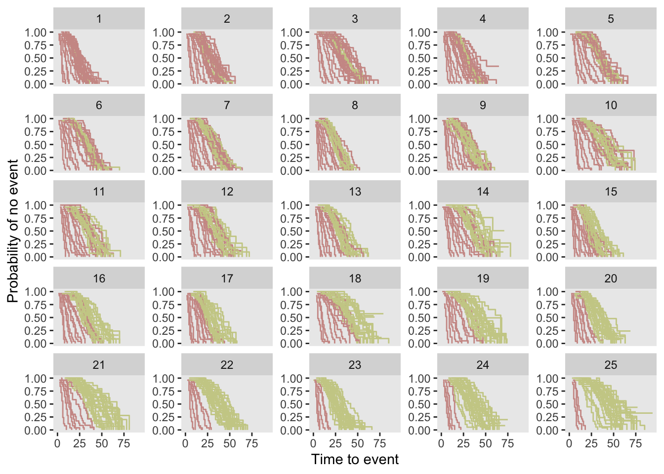
dd <- dd[, .(id, site, k, A, Y, event)]

Model estimation

This model has quite a few components relative to the earlier models, but nothing is really new. There is a penalized spline for the effect of time and a random effect for each site. The primary parameter of interest is still $\beta$.

For completeness, here is the model specification:

$\log L(\beta) = \sum_{j=1}^{J} \left[ \sum_{i \in D_j} \left(\beta A_i + \sum_{m=1} ^ M \gamma_m X_{m_i} + b_{s[i]} \right) - \sum_{r=0}^{d_j-1} \log \left( \sum_{k \in R_j} \left(\beta A_k + \sum_{m=1} ^ M \gamma_m X_{m_i} + b_{s[k]} \right) - r \cdot \bar{w}_j \right) \right] - \lambda \sum_{m=1}^{M} \left( Q^{(2)} \gamma \right)_m^2 \\$

where

• $J$: number of unique event times
• $M$: number of spline basis functions
• $D_j$ is the set of individuals who experience an event at time $t_j$.
• $R_j$ is the risk set at time $t_j$, including all individuals who are still at risk at that time.
• $d_j$ is the number of events occurring at time $t_j$.
• $r$ ranges from 0 to $d_j - 1$, iterating over the tied events.
• $\bar{w}_j$ represents the average risk weight of individuals experiencing an event at $t_j$:

$\bar{w}_j = \frac{1}{d_j} \sum_{i \in D_j} \left(\beta A_i + b_{s[i]} \right)$

• $A_i$: binary indicator for treatment
• $X_{m_i}$: value of the $m^{\text{th}}$ spline basis function for the $i^{\text{th}}$ observation
• $Q^{(2)}$: the second-difference matrix of the spline function

The parameters of the model are

• $\beta$: treatment coefficient
• $\gamma_m$: spline coefficient for the $m^\text{th}$ spline basis function
• $b_{s[i]}$: cluster-specific random effect, where $s[i]$ is the cluster of patient $i$
• $\lambda$: the penalization term; this will not be estimated but provided by the user

The assumed prior distributions for $\beta$ and the random effects are:

$\begin{aligned} \beta &\sim N(0,4) \\ b_i &\sim N(0,\sigma_b) \\ \sigma_b &\sim t_{\text{student}}(df = 3, \mu=0, \sigma = 2) \\ \gamma_m &\sim N(0,2) \end{aligned}$

And here is the implementation of the model in Stan:

stan_code <- 
"
data {
  
  int<lower=1> S;          // Number of clusters
  int<lower=1> K;          // Number of covariates
  
  int<lower=1> N_o;        // Number of uncensored observations
  array[N_o] int i_o;      // Event times (sorted in decreasing order)

  int<lower=1> N;          // Number of total observations
  matrix[N, K] x;          // Covariates for all observations
  array[N] int<lower=1,upper=S> s;          // Cluster
  
  // Spline-related data
  
  int<lower=1> Q;          // Number of basis functions
  matrix[N, Q] B;          // Spline basis matrix
  matrix[N, Q] Q2_spline;  // 2nd derivative for penalization
  real<lower=0> lambda;    // penalization term
  
  array[N] int index;

  int<lower=0> T;            // Number of records as ties
  int<lower=1> J;            // Number of groups of ties
  array[T] int t_grp;        // Indicating tie group
  array[T] int t_index;      // Index in data set
  vector[T] t_adj;           // Adjustment for ties (efron)
  
}

parameters {
  
  vector[K] beta;          // Fixed effects for covariates
  
  vector[S] b;             // Random effects
  real<lower=0> sigma_b;   // SD of random effect
  
  vector[Q] gamma;         // Spline coefficients
  
}

model {
  
  // Priors
  
  beta ~ normal(0, 1);
  
  // Random effects
  
  b ~ normal(0, sigma_b);
  sigma_b ~ normal(0, 0.5);

  
  // Spline coefficients prior
  
  gamma ~ normal(0, 2);
  
  // Penalization term for spline second derivative
  
  target += -lambda * sum(square(Q2_spline * gamma));
  
  // Compute cumulative sum of exp(theta) in log space (more efficient)
  
  vector[N] theta;
  vector[N] log_sum_exp_theta;
  vector[J] exp_theta_grp = rep_vector(0, J);
  
  int first_in_grp;
  
  // Calculate theta for each observation
  
  for (i in 1:N) {
    theta[i] = dot_product(x[i], beta) + dot_product(B[i], gamma) + b[s[i]];
  }
  
  // Compute cumulative sum of log(exp(theta)) from last to first observation
  
  log_sum_exp_theta = rep_vector(0.0, N);
  log_sum_exp_theta[N] = theta[N];
  
  for (i in tail(sort_indices_desc(index), N-1)) {
    log_sum_exp_theta[i] = log_sum_exp(theta[i], log_sum_exp_theta[i + 1]);
  }

   // Efron algorithm - adjusting cumulative sum for ties
  
  for (i in 1:T) {
    exp_theta_grp[t_grp[i]] += exp(theta[t_index[i]]);
  }

  for (i in 1:T) {
  
    if (t_adj[i] == 0) {
      first_in_grp = t_index[i];
    }

    log_sum_exp_theta[t_index[i]] =
      log( exp(log_sum_exp_theta[first_in_grp]) - t_adj[i] * exp_theta_grp[t_grp[i]]);
  }
  
  // Likelihood for uncensored observations

  for (n_o in 1:N_o) {
    target += theta[i_o[n_o]] - log_sum_exp_theta[i_o[n_o]];
  }
}
"

Compiling the model:

stan_model <- cmdstan_model(write_stan_file(stan_code))

Getting the data from R to Stan:

dx <- copy(dd)
setorder(dx, Y)
dx[, index := .I]

dx.obs <- dx[event == 1]
N_obs <- dx.obs[, .N]
i_obs <- dx.obs[, index]

N_all <- dx[, .N]
x_all <- data.frame(dx[, .(A)])
s_all <- dx[, site]

K <- ncol(x_all)                 # num covariates - in this case just A
S <- dx[, length(unique(site))]

# Spline-related info

n_knots <- 5
spline_degree <- 3
knot_dist <- 1/(n_knots + 1)
probs <- seq(knot_dist, 1 - knot_dist, by = knot_dist)
knots <- quantile(dx$k, probs = probs)
spline_basis <- bs(dx$k, knots = knots, degree = spline_degree, intercept = TRUE)
B <- as.matrix(spline_basis)

Q2 <- dbs(dx$k, knots = knots, degree = spline_degree, derivs = 2, intercept = TRUE)
Q2_spline <- as.matrix(Q2)

ties <- dx[, .N, keyby = Y][N>1, .(grp = .I, Y)]
ties <- merge(ties, dx, by = "Y")
ties <- ties[, order := 1:.N, keyby = grp][, .(grp, index)]
ties[, adj := 0:(.N-1)/.N, keyby = grp]

stan_data <- list(
  S = S,
  K = K,
  N_o = N_obs,
  i_o = i_obs,
  N = N_all,
  x = x_all,
  s = s_all,
  Q = ncol(B),
  B = B,
  Q2_spline = Q2_spline,
  lambda = 0.15,
  index = dx$index,
  T = nrow(ties),
  J = max(ties$grp),
  t_grp = ties$grp,
  t_index = ties$index,
  t_adj = ties$adj
)

Now we sample from the posterior - you can see that it takes quite a while to run, at least on my 2020 MacBook Pro M1 with 8GB RAM:

fit_mcmc <- stan_model$sample(
  data = stan_data,
  seed = 1234,
  iter_warmup = 1000,
  iter_sampling = 4000,
  chains = 4,
  parallel_chains = 4,
  refresh = 0
)

## Running MCMC with 4 parallel chains...

## Chain 4 finished in 1847.8 seconds.
## Chain 1 finished in 2202.8 seconds.
## Chain 3 finished in 2311.8 seconds.
## Chain 2 finished in 2414.9 seconds.
## 
## All 4 chains finished successfully.
## Mean chain execution time: 2194.3 seconds.
## Total execution time: 2415.3 seconds.

fit_mcmc$summary(variables = c("beta", "sigma_b"))

## # A tibble: 2 × 10
##   variable  mean median     sd    mad    q5   q95  rhat ess_bulk ess_tail
##   <chr>    <dbl>  <dbl>  <dbl>  <dbl> <dbl> <dbl> <dbl>    <dbl>    <dbl>
## 1 beta[1]  0.815  0.815 0.0298 0.0298 0.767 0.865  1.00    3513.    5077.
## 2 sigma_b  0.543  0.535 0.0775 0.0739 0.432 0.683  1.00    3146.    5110.

Estimating a “frequentist” random-effects model

After all that, it turns out you can just fit a frailty model with random effects for site and a spline for time period $k$ using the coxmme package. This is obviously much simpler then everything I have presented here.

frailty_model <- coxme(Surv(Y, event) ~ A + ns(k, df = 3) + (1 | site), data = dd)
summary(frailty_model)

## Mixed effects coxme model
##  Formula: Surv(Y, event) ~ A + ns(k, df = 3) + (1 | site) 
##     Data: dd 
## 
##   events, n = 14989, 18750
## 
## Random effects:
##   group  variable        sd  variance
## 1  site Intercept 0.5306841 0.2816256
##                   Chisq    df p   AIC   BIC
## Integrated loglik 18038  5.00 0 18028 17990
##  Penalized loglik 18185 27.85 0 18129 17917
## 
## Fixed effects:
##                    coef exp(coef) se(coef)      z      p
## A               0.80966   2.24714  0.02959  27.36 <2e-16
## ns(k, df = 3)1 -2.71392   0.06628  0.04428 -61.29 <2e-16
## ns(k, df = 3)2  1.04004   2.82933  0.07851  13.25 <2e-16
## ns(k, df = 3)3  4.48430  88.61492  0.04729  94.83 <2e-16

However, the advantage of the Bayesian model is its flexibility. For example, if you wanted to include site-specific spline curves—analogous to site-specific time effects—you could extend the Bayesian approach to do so. The current Bayesian model implements a study-wide time spline, but incorporating site-specific splines would be a natural extension. I initially hoped to implement site-specific splines using the mgcv package, but the models did not converge. I am quite confident that a Bayesian extension would, though it would likely require substantial computing resources. If someone wants me to try that, I certainly could, but for now, I’ll stop here.