A Bayesian proportional hazards model for a cluster randomized trial

Simulating data with a cluster-specific random effect

Here are the R packages used in the post:

library(simstudy)
library(ggplot2)
library(data.table)
library(survival)
library(survminer)
library(cmdstanr)

The dataset simulates a cluster randomized trial where sites are randomized in a $1:1$ ratio to either the treatment group ($A=1$) or control group ($A=0$). Patients are affiliated with sites and receive the intervention based on site-level randomization. The time-to-event outcome, $Y$, is measured at the patient level and depends on both the site’s treatment assignment and unmeasured site effects:

defC <- 
  defData(varname = "b", formula = 0, variance = "..s2_b", dist = "normal") |>
  defData(varname = "A", formula = "1;1", dist = "trtAssign")

defS <-
  defSurv(
    varname = "timeEvent",
    formula = "-11.6 + ..delta_f * A + b",
    shape = 0.30
  )  |>
  defSurv(varname = "censorTime", formula = -11.3, shape = .40)

delta_f <- 0.7
s2_b <- 0.4^2

I’ve generated a single data set of 50 sites, with 25 in each arm. Each site includes 100 patients. The plot below shows the site-specific Kaplan-Meier curves for each intervention arm.

set.seed(1821)

dc <- genData(50, defC, id = "site")
dd <- genCluster(dc, "site", numIndsVar = 100, level1ID = "id")
dd <- genSurv(dd, defS, timeName = "Y", censorName = "censorTime",
             eventName = "event", typeName = "eventType", keepEvents = TRUE)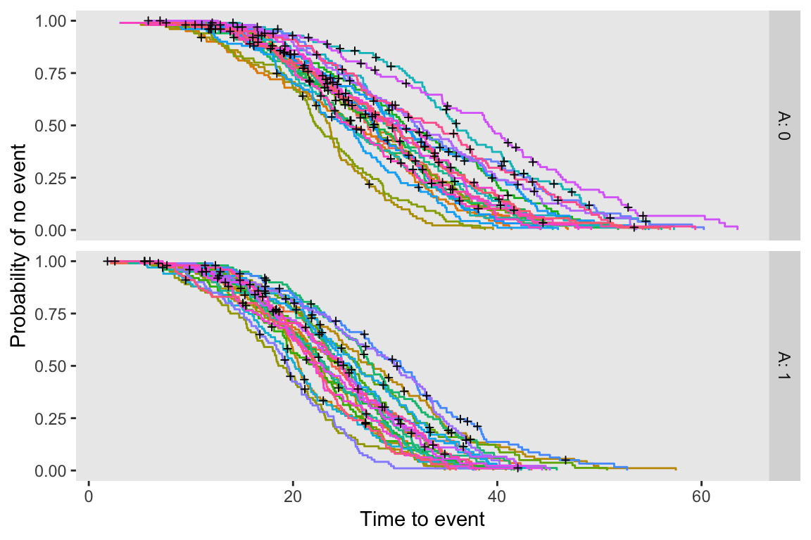

Bayesian model

Since this is the fourth iteration of the Bayesian proportional hazards model I’ve been working on, it naturally builds directly on the approach from my previous three posts (here. here, and here). Now, the partial log likelihood is a function of the treatment effect and cluster-specific random effects, given by:

$\log L(\beta) = \sum_{j=1}^{J} \left[ \sum_{i \in D_j} \left(\beta A_i + b_{s[i]} \right) - \sum_{r=0}^{d_j-1} \log \left( \sum_{k \in R_j} \left(\beta A_k + b_{s[k]} \right) - r \cdot \bar{w}_j \right) \right] \\$

where

• $J$: number of unique event times
• $D_j$ is the set of individuals who experience an event at time $t_j$.
• $R_j$ is the risk set at time $t_j$, including all individuals who are still at risk at that time.
• $d_j$ is the number of events occurring at time $t_j$.
• $r$ ranges from 0 to $d_j - 1$, iterating over the tied events.
• $\bar{w}_j$ represents the average risk weight of individuals experiencing an event at $t_j$:

$\bar{w}_j = \frac{1}{d_j} \sum_{i \in D_j} \left(\beta A_i + b_{s[i]} \right)$

• $A_i$: binary indicator for treatment for patient $i$.

The parameters of the model are

• $\beta$: treatment coefficient
• $b_{s[i]}$: cluster-specific random effect, where $s[i]$ is the cluster of patient $i$

The assumed prior distributions for $\beta$ and the random effects are:

$\begin{aligned} \beta &\sim N(0,4) \\ b_i &\sim N(0,\sigma_b) \\ \sigma_b &\sim t_{\text{student}}(df = 3, \mu=0, \sigma = 2) \end{aligned}$

stan_code <- 
"
data {
  
  int<lower=0> S;                   // Number of clusters

  int<lower=0> K;                   // Number of covariates
  int<lower=0> N_o;                 // Number of uncensored observations
  array[N_o] int i_o;               // Index in data set

  int<lower=0> N;                   // Number of total observations
  matrix[N, K] x;                   // Covariates for all observations
  array[N] int<lower=1,upper=S> s;  // Cluster for each observation
  
  array[N] int index;
  
  int<lower=0> T;            // Number of records as ties
  int<lower=1> J;            // Number of groups of ties
  array[T] int t_grp;        // Indicating tie group
  array[T] int t_index;      // Index in data set
  vector[T] t_adj;           // Adjustment for ties (efron)

}

parameters {
  
  vector[K] beta;          // Fixed effects for covariates
  vector[S] b;             // Random effects
  real<lower=0> sigma_b;   // Variance of random effect
  
}

model {
  
  // Prior
  
  beta ~ normal(0, 4);
  b ~ normal(0, sigma_b);
  sigma_b ~ student_t(3, 0, 2);
  
  // Calculate theta for each observation to be used in likelihood
  
  vector[N] theta;
  vector[N] log_sum_exp_theta;
  vector[J] exp_theta_grp = rep_vector(0, J);
  
  int first_in_grp;

  
  for (i in 1:N) {
    theta[i] = dot_product(x[i], beta) + b[s[i]];  
  }
  
  // Computing cumulative sum of log(exp(theta)) from last to first observation
  
  log_sum_exp_theta[N] = theta[N];
  
  for (i in tail(sort_indices_desc(index), N-1)) {
    log_sum_exp_theta[i] = log_sum_exp(theta[i], log_sum_exp_theta[i + 1]);
  }

  // Efron algorithm - adjusting cumulative sum for ties
  
  for (i in 1:T) {
    exp_theta_grp[t_grp[i]] += exp(theta[t_index[i]]);
  }

  for (i in 1:T) {
  
    if (t_adj[i] == 0) {
      first_in_grp = t_index[i];
    }

    log_sum_exp_theta[t_index[i]] =
      log( exp(log_sum_exp_theta[first_in_grp]) - t_adj[i] * exp_theta_grp[t_grp[i]]);
  }
  
  // Likelihood for uncensored observations

  for (n_o in 1:N_o) {
    target += theta[i_o[n_o]] - log_sum_exp_theta[i_o[n_o]];
  }
}
"

Getting the data ready to pass to Stan, compiling the Stan code, and sampling from the model using cmdstanr:

dx <- copy(dd)
setorder(dx, Y)
dx[, index := .I]

dx.obs <- dx[event == 1]
N_obs <- dx.obs[, .N]
i_obs <- dx.obs[, index]

N_all <- dx[, .N]
x_all <- data.frame(dx[, .(A)])
s_all <- dx[, site]

K <- ncol(x_all)                 # num covariates - in this case just A
S <- dx[, length(unique(site))]

ties <- dx[, .N, keyby = Y][N>1, .(grp = .I, Y)]
ties <- merge(ties, dx, by = "Y")
ties <- ties[, order := 1:.N, keyby = grp][, .(grp, index)]
ties[, adj := 0:(.N-1)/.N, keyby = grp]

stan_data <- list(
  S = S,
  K = K,
  N_o = N_obs,
  i_o = i_obs,
  N = N_all,
  x = x_all,
  s = s_all,
  index = dx$index,
  T = nrow(ties),
  J = max(ties$grp),
  t_grp = ties$grp,
  t_index = ties$index,
  t_adj = ties$adj
)

# compiling code

stan_model <- cmdstan_model(write_stan_file(stan_code))

# sampling from model

fit <- stan_model$sample(
  data = stan_data,
  seed = 1234, 
  iter_warmup = 1000,
  iter_sampling = 4000,
  chains = 4,
  parallel_chains = 4,
  refresh = 0
)

## Running MCMC with 4 parallel chains...

## Chain 3 finished in 39.0 seconds.
## Chain 2 finished in 39.1 seconds.
## Chain 1 finished in 39.5 seconds.
## Chain 4 finished in 39.5 seconds.
## 
## All 4 chains finished successfully.
## Mean chain execution time: 39.3 seconds.
## Total execution time: 39.7 seconds.

The posterior mean for $\beta$, the treatment effect, is quite close to the “true” value of 0.70, as is the estimate of the standard deviation of the random effect (we used $sd = 0.4$ in the data generating process):

fit$summary(variables = c("beta", "sigma_b"))

## # A tibble: 2 × 10
##   variable  mean median     sd    mad    q5   q95  rhat ess_bulk ess_tail
##   <chr>    <dbl>  <dbl>  <dbl>  <dbl> <dbl> <dbl> <dbl>    <dbl>    <dbl>
## 1 beta[1]  0.659  0.660 0.124  0.124  0.455 0.863  1.00    1529.    3265.
## 2 sigma_b  0.417  0.413 0.0472 0.0458 0.347 0.501  1.00   15493.   11171.

The final post in this series will include code to simulate data from a stepped-wedge cluster-randomized trial with a time-to-event outcome. This model will integrate both the spline and random effect components. I’m curious to see how well it performs, as the required computational resources could be substantial.