I’ve been curious to see how helpful ChatGPT can be for implementing relatively complicated models in R. About two years ago, I described a model for estimating a treatment effect in a cluster-randomized stepped wedge trial. We used a generalized additive model (GAM) with site-specific splines to account for general time trends, implemented using the mgcv package. I’ve been interested in exploring a Bayesian version of this model, but hadn’t found the time to try - until I happened to pose this simple question to ChatGPT:
I want to build an R Stan model with cluster specific random splines - is that possible?
And as ChatGPT does, it eagerly let me know that this would not be a problem:
Yes, it’s possible to build a model in R using Stan with cluster-specific random splines. This approach involves using a hierarchical model where each cluster has its own spline, but the splines share a common structure.
Here is a step-by-step outline to guide you through this process:
- Data Preparation: Organize your data into clusters and ensure it’s in a suitable format for modeling.
- Spline Basis Functions: Generate spline basis functions (e.g., B-splines) for your data. This can be done using packages like
splinesormgcvin R.- Stan Model Code: Write the Stan code for the hierarchical spline model. The model will include cluster-specific random effects for the spline coefficients.
- Data List for Stan: Create a list of data inputs required by the Stan model, including the spline basis functions and the data itself.
- Run the Model: Use the
rstanpackage to compile and fit the model.
Maybe I shouldn’t have been, but I was pretty impressed by the code that followed. What follows are the highlights of my interaction with ChatGPT.
Preliminaries
Before getting started, here are the libraries needed to run all of the following code:
library(ggplot2)
library(simstudy)
library(data.table)
library(mgcv)
library(splines)
library(splines2)
library(cmdstanr)
library(posterior)
Data generation
To explore different modeling options, I wanted a simple data generation process to create the simulated data set. ChatGPT suggested using the following non-linear function for , the outcome for individual in cluster , based on predictor : The code was simple enough:
set.seed(2024)

n <- 1000
k <- 10  # number of clusters
x <- runif(n)
cluster <- sample(1:k, n, replace = TRUE)
y <- sin(2  * pi * x) + rnorm(n, sd = 0.35)
dd <- data.table(y, x, cluster)
dd$cluster <- factor(dd$cluster)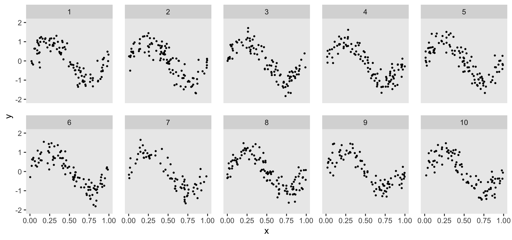
Although the data generation process suggested by ChatGPT was helpful, it had a significant shortcoming. I wanted to model cluster-specific spline curves, but the ChatGPT code generated the same curve for all clusters. To address this, I used the general formulation and added a cluster-specific effect , which stretches the sin curve differently for each cluster:
k <- 10  # number of clusters

defc <- defData(varname = "a", formula = "0.6;1.4", dist = "uniform")
defi <-
  defDataAdd(varname = "x", formula = "0;1", dist = "uniform") |>
  defDataAdd(
    varname = "y",
    formula =  "sin(2 * a * ..pi * x)",
    variance = 0.35^2
  )

dc <- genData(k, defc, id = "cluster")
dd <- genCluster(dc, "cluster", 100, "id")
dd <- addColumns(defi, dd)
dd[, cluster := factor(cluster)]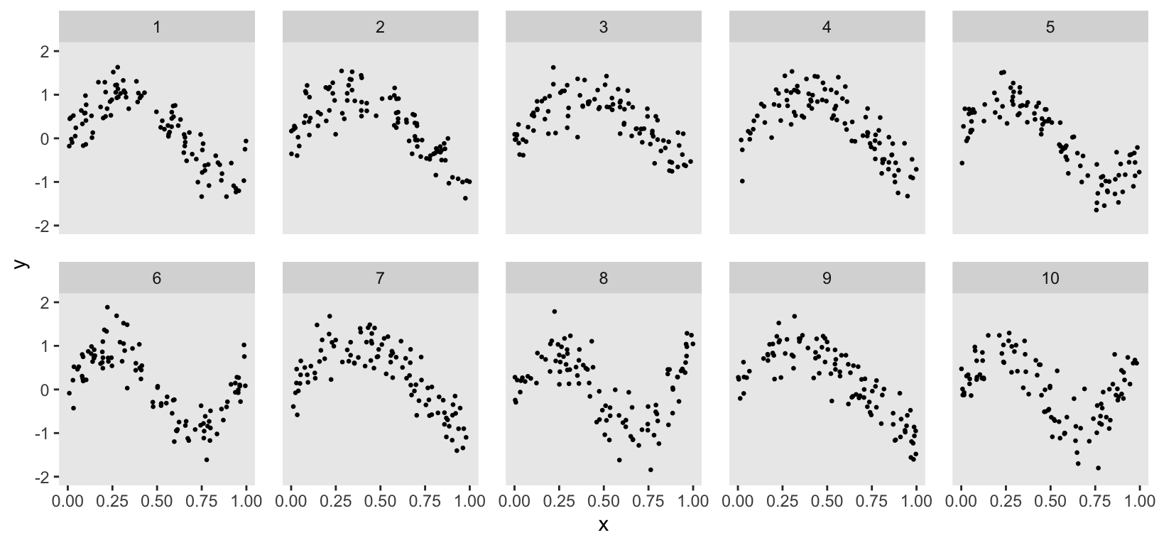
Data modeling
The goal is to estimate cluster-specific curves that capture the relationship between and within each cluster. I am aiming for these curves to reflect the overall trend without overfitting the data; in other words, we want the estimated function to provide a smooth and interpretable representation of the relationship, balancing flexibility and simplicity.
Although the purpose of my conversation with ChatGPT was to get a Bayesian version of this random spline model, I started off by asking for it to generate a generalized additive model (GAM) to provide a basis for comparison. This is what it came up with:
where is a smooth spline function of . The estimated model can be used to provide predictions that can be plotted to describe the relationship between and :
gam <- gamm(
  y ~ s(x) + s(x, cluster, bs = "fs", k = 8),
  data = dd, method="REML"
)

dd$g <- predict(gam$gam)
Bayesian spline model
The first Bayesian model that ChatGPT generated can be described using this notation:
Data
- : number of individuals
- : number of clusters
- : number of spline basis functions
- : outcome for individual in cluster , ,
- : matrix of spline basis function values
Parameters
- : spline coefficients for cluster (a vector of length for each cluster)
- : standard deviation of the observation noise
- : prior standard deviation for the spline coefficients
Model
Likelihood:
Priors:
The Stan code provided by ChatGPT aligns with this description. As part of the model, I also requested code to generate outcome predictions for each observation, which is implemented in the generated quantities block. My goal was to plot the median of those predictions for each individual as a comparison to the GAM plot above.”
data {
  int<lower=1> N;                          // number of observations
  int<lower=1> K;                          // number of clusters
  int<lower=1> M;                          // number of basis functions
  array[N] int<lower=1, upper=K> cluster;  // cluster ids
  matrix[N, M] X_spline;                   // basis function values
  vector[N] y;                             // response variable
}

parameters {
  matrix[K, M] beta;          // cluster-specific spline coefficients
  real<lower=0> sigma_y;      // observation noise
  real<lower=0> sigma_beta;   // prior standard deviation for beta
}

model {
  sigma_y ~ normal(0, 1);
  sigma_beta ~ normal(0, 1);

  // Priors for beta

  for (k in 1:K) {
    beta[k] ~ normal(0, sigma_beta);
  }

  // Likelihood

  for (n in 1:N) {
    y[n] ~ normal(X_spline[n] * beta[cluster[n]]', sigma_y);
  }
}

generated quantities {

  vector[N] y_pred;                    // Vector of observations.

  for (n in 1:N) {
    y_pred[n] = normal_rng(X_spline[n] * beta[cluster[n]]', sigma_y);
  }
}
Spline basis functions
In the likelihood, is modeled as a function of the vector rather than the single measurement . While I won’t delve deeply into spline estimation, I want to conceptually outline how this vector is constructed in the context of cubic splines.
We control the flexibility of the curve by specifying the number of knots. A unique curve is fitted between each pair of knots (as well as at the ends), with constraints ensuring smooth transitions between these curves. The estimation of these curves is performed using basis functions, specifically B-spline basis functions of .
The number of basis functions is determined by the number of knots. For instance, the plot below illustrates the basis functions required for knots. Each basis function contributes an element to the vector for each value of . In the case of cubic splines, at most four basis functions can be non-zero between any two knots, as indicated by the intervals on the x-axis. Consequently, the vector consists of the values of each basis function at a given point , with at most four non-zero entries corresponding to the active basis functions. (As an example, in the plot below there is a vertical line at a single point that passes through four basis functions.)
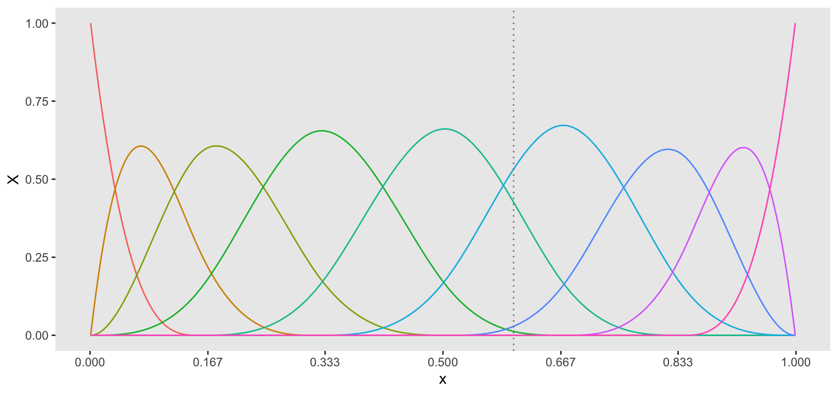
This example uses knots to introduce a slight overfitting of the data, which will allow me to apply another model in the next step that will further smooth the curves. (In a real-world setting, it may have made more sense to start out with fewer knots.) The bs function (in the splines package) computes the B-spline basis function values for each observed .
n_knots <- 5
knot_dist <- 1/(n_knots + 1)
probs <- seq(knot_dist, 1 - knot_dist, by = knot_dist)
knots <- quantile(dd$x, probs = probs)
spline_basis <- bs(dd$x, knots = knots, degree = 3, intercept = TRUE)
X_spline <- as.matrix(spline_basis)
Data list for stan
To fit the model, we need to create the data set that Stan will use to estimate the parameters.
stan_data <- list(
  N = nrow(dd),           # number of observations
  K = k,                  # number of clusters
  M = ncol(X_spline),     # number of basis functions
  cluster = dd$cluster,   # vector of cluster ids
  X_spline = X_spline,    # basis function values
  y = dd$y                # response variable
)
Run stan model
ChatGPT provided code to estimate the model using the rstan package. However, I prefer using the cmdstanr package, which I find more stable and generally less finicky. From the plot, you can see that the estimation was quite good. However, the curves are a bit too wiggly, indicating the data may have been slightly overfit, particularly for clusters 1, 3, and 7.
mod <- cmdstan_model("code/spline.stan")

fit <- mod$sample(
  data = stan_data,
  chains = 4,
  iter_warmup = 500,
  iter_sampling = 2000,
  parallel_chains = 4,
  refresh = 0 # print update every 500 iters
)
## Running MCMC with 4 parallel chains...## Chain 2 finished in 5.4 seconds.
## Chain 1 finished in 5.6 seconds.
## Chain 3 finished in 5.6 seconds.
## Chain 4 finished in 5.8 seconds.
##
## All 4 chains finished successfully.
## Mean chain execution time: 5.6 seconds.
## Total execution time: 5.9 seconds.draws <- as_draws_df(fit$draws())
ds <- summarize_draws(draws, .fun = median) |> data.table()
dd$np <- ds[substr(variable, 1, 3) == "y_p", 2]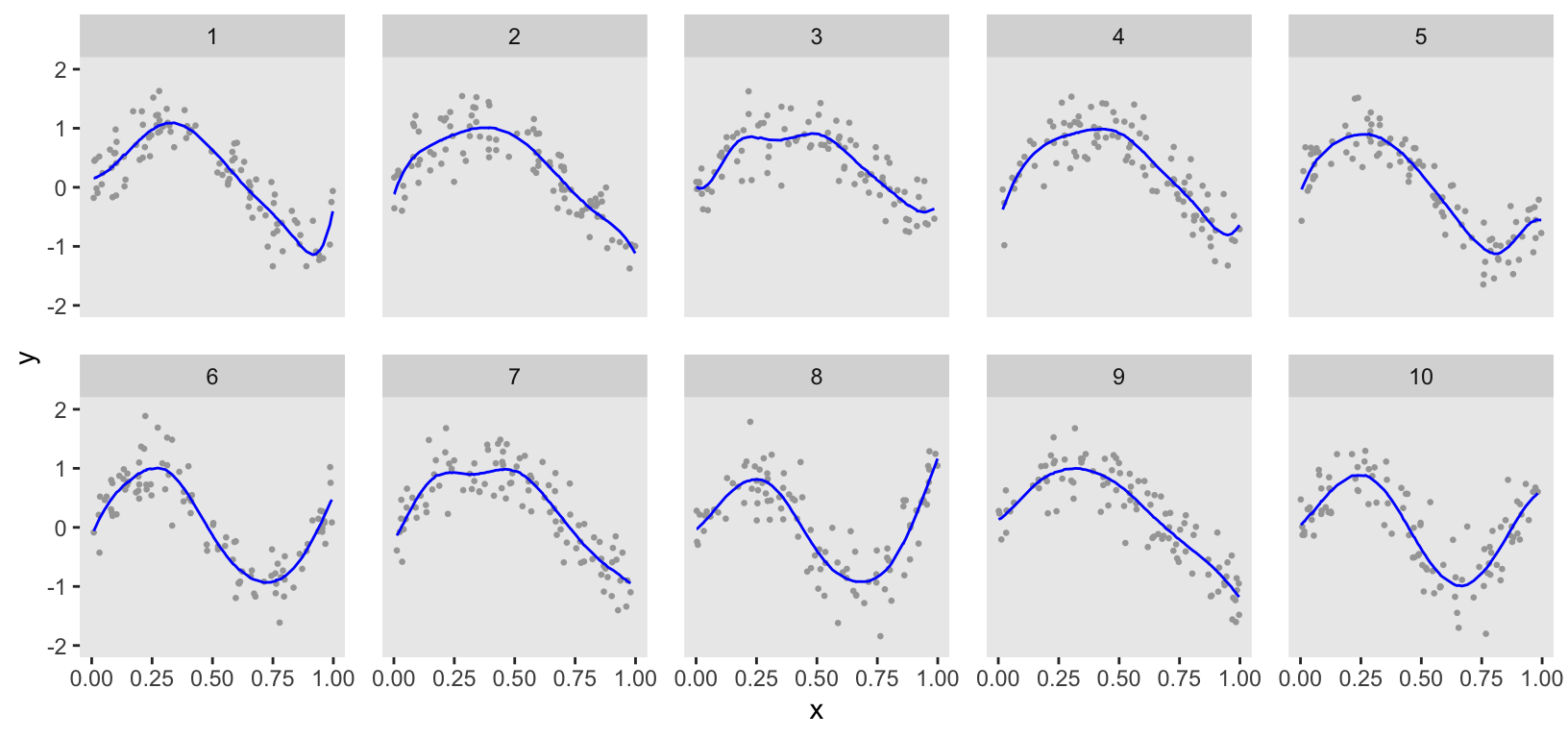
Penalized spline
When I made my initial inquiry to ChatGPT, it provided only a single model and didn’t indicate that there might be alternatives. To elicit another option, I had to specifically ask. To smooth the estimate provided by the initial model (which admittedly I made too wiggly on purpose), I asked ChatGPT to provide a penalized Bayesian spline model, and it obliged.
The model is just an extension of the spline model, with an added penalization term that is based on the second derivative of the B-spline basis functions. We can strengthen or weaken the penalization term using a tuning parameter , that is provided to the model. The Stan model code is unchanged from the original model, except for the added penalization term.
model {

  sigma_y ~ normal(0, 1);
  sigma_beta ~ normal(0, 1);

  // Priors for beta

  for (k in 1:K) {
    beta[k] ~ normal(0, sigma_beta);
  }

  //Penalization <---------------------------------------

  for (k in 1:K) {
    target += -lambda * sum(square(D2_spline * beta[k]'));
  }

  // Likelihood

  for (n in 1:N) {
    y[n] ~ normal(X_spline[n] * beta[cluster[n]]', sigma_y);
  }
}
The second derivatives of the B-spline basis functions are estimated using the dbs function in the splines2 package. Like the matrix , has dimensions . Both and are added to the data passed to Stan:
D2 <- dbs(dd$x, knots = knots, degree = 3, derivs = 2, intercept = TRUE)
D2_spline <- as.matrix(D2)

stan_data <- list(
  N = nrow(dd),
  K = k,
  M = ncol(X_spline),
  cluster = dd$cluster,
  X_spline = X_spline,
  D2_spline = D2_spline,
  y = dd$y,
  lambda = 0.00005
)
## Running MCMC with 4 parallel chains...## Chain 2 finished in 16.5 seconds.
## Chain 1 finished in 16.6 seconds.
## Chain 3 finished in 16.7 seconds.
## Chain 4 finished in 16.7 seconds.
##
## All 4 chains finished successfully.
## Mean chain execution time: 16.6 seconds.
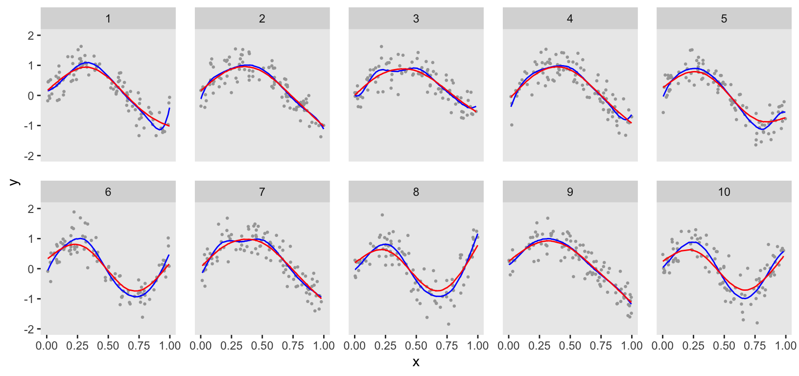
## Total execution time: 16.8 seconds.The plot directly comparing the penalized Bayesian model with the initial Bayesian model (initial Bayesian model in blue) shows the impact of further smoothing.
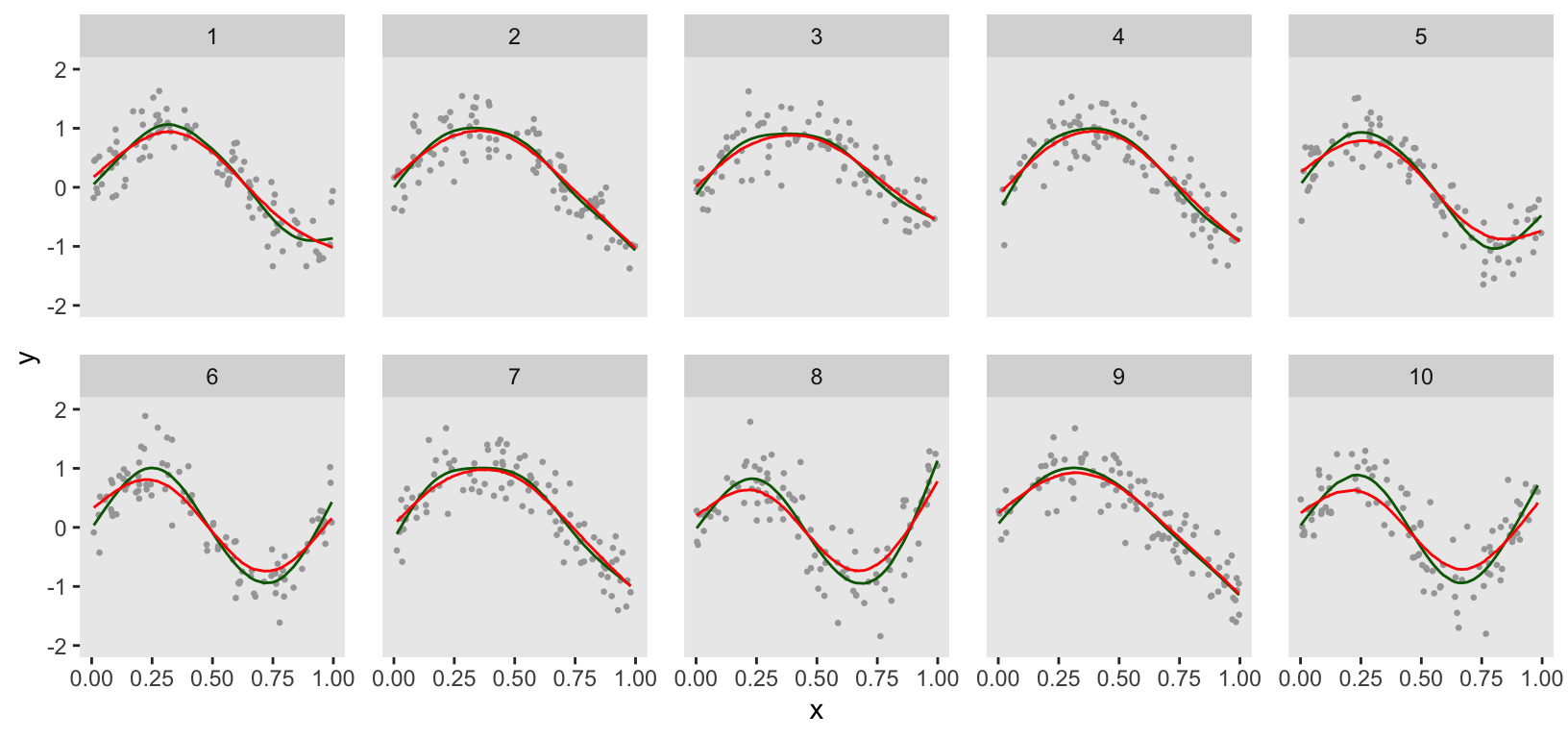
A direct comparison between the GAM and penalized Bayesian models (GAM in green) suggests that there might be some differences in the estimation for at least several clusters, particularly those that change direction twice. The penalized Bayesian model appears to be smoothing more than the GAM:
I was also aware of a third version of the Bayesian spline model that uses a random-walk prior on the to induce smoothing. Unprompted, ChatGPT did not mention this. But, upon request it did give me code that I was able to implement successfully. I’ll leave it to you to explore this further on your own—or perhaps ask ChatGPT for assistance.
Reference:
OpenAI. (2024). ChatGPT (September 30, Version) [Large language model]. https://chat.openai.com/
Support:
This work is supported within the National Institutes of Health (NIH) Health Care Systems Research Collaboratory by cooperative agreement UG3/UH3AT009844 from the National Institute on Aging. This work also received logistical and technical support from the NIH Collaboratory Coordinating Center through cooperative agreement U24AT009676. Support was also provided by the NIH National Center for Complementary and Integrative Health Administrative Supplement for Complementary Health Practitioner Research Experience through cooperative agreement UH3AT009844 and by the National Center for Complementary and Integrative Health of the National Institutes of Health under award number UH3AT009844. Work also supported by Memorial Sloan Kettering Cancer Center Support Grant/Core Grant P30CA008748. The author was the sole writer of this blog post and has no conflicts. The content is solely the responsibility of the author and does not necessarily represent the official views of the National Institutes of Health.