A researcher reached out to me a few weeks ago. They were trying to generate longitudinal data that included irregularly spaced follow-up periods. The default periods generated by the function addPeriods in the simstudy package are \(\{0, 1, 2, ..., n - 1\}\), where there are \(n\) total periods. However, when follow-up periods required more specificity, such as \(\{0, 90, 180, 365\}\) days from baseline, users had to manually add them. Originally, I had intended to incorporate this feature into the function, but unfortunately it slipped through the cracks. Thanks to the clear motivation provided by the researcher, I’ve implemented this enhancement. Users can now replace the default vector with their desired set of follow-up periods using the new argument periodVec. This addition is available in the development version of simstudy on GitHub.
Just as a quick introduction, here is a simple example that shows the default settings of addPeriods. We are generating three individuals that will have measurements at four different periods, generically identified as \(\{0, 1, 2, 3\}\):
library(simstudy)
set.seed(123)

dd <- genData(3)
dp <- addPeriods(dd, nPeriods = 4)
## Key: <timeID>
## id period timeID
## <int> <int> <int>
## 1: 1 0 1
## 2: 1 1 2
## 3: 1 2 3
## 4: 1 3 4
## 5: 2 0 5
## 6: 2 1 6
## 7: 2 2 7
## 8: 2 3 8
## 9: 3 0 9
## 10: 3 1 10
## 11: 3 2 11
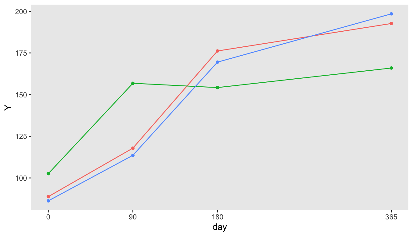
## 12: 3 3 12In this next example, we still assume four measurement periods, but they will be at baseline, 90 days, 180 days, and 1 year. The outcome \(Y\) that is a function of the day of follow-up:
def <- defDataAdd(varname = "Y", formula = "100 + 0.25 * day", variance = 400)

dd <- genData(3)
dp <- addPeriods(dd, nPeriods = 4, perName = "day", periodVec = c(0, 90, 180, 365))
dp <- addColumns(def, dp)
Here is the resulting data set:
## Key: <timeID>
##        id   day timeID         Y
##     <int> <num>  <int>     <num>
##  1:     1     0      1  88.79049
##  2:     1    90      2 117.89645
##  3:     1   180      3 176.17417
##  4:     1   365      4 192.66017
##  5:     2     0      5 102.58575
##  6:     2    90      6 156.80130
##  7:     2   180      7 154.21832
##  8:     2   365      8 165.94878
##  9:     3     0      9  86.26294
## 10:     3    90     10 113.58676
## 11:     3   180     11 169.48164
## 12:     3   365     12 198.44628
The second example transforms data in “wide” format to “long” format. Here is the wide data generation:
tdef <-
  defData(varname = "Y0", dist = "normal", formula = 10, variance = 1) |>
  defData(varname = "Y1", dist = "normal", formula = "Y0 + 5", variance = 1) |>
  defData(varname = "Y2", dist = "normal", formula = "Y0 + 10", variance = 1)

dd <- genData(3, tdef)
## Key: <id>
## id Y0 Y1 Y2
## <int> <num> <num> <num>
## 1: 1 10.400771 17.18768 21.10213
## 2: 2 10.110683 15.60853 19.63789
## 3: 3 9.444159 12.47754 18.37634And here is the transformation, with the time periods:
dp <- addPeriods(
  dd,
  perName = "day",
  timevars = paste0("Y", 0:2),
  timevarName = "Y",
  periodVec = c(0, 180, 365)
)
## Key: <timeID>
## id day Y timeID
## <int> <num> <num> <int>
## 1: 1 0 10.400771 1
## 2: 1 180 17.187685 2
## 3: 1 365 21.102127 3
## 4: 2 0 10.110683 4
## 5: 2 180 15.608533 5
## 6: 2 365 19.637891 6
## 7: 3 0 9.444159 7
## 8: 3 180 12.477542 8
## 9: 3 365 18.376335 9As a little bonus, here is additional code to introduce a little more reality into the data generation process. In this case, not all the follow-up measurements would be collected precisely on the exact follow-up date (although all the baseline measurements would be made on day zero). In particular, we are assuming that about 60% of the cases would be collected after the scheduled time (never before). I’ve implemented this logic by creating a lag variable in the data definition:
deflag <-
  defDataAdd(varname = "lagdays", formula = 10, dist = "noZeroPoisson") |>
  defDataAdd(varname = "lag", formula = "0 | .4 + lagdays | .6", dist = "mixture") |>
  defDataAdd(varname = "obs_day", formula = "(day > 0) * (day + lag)")

dd <- genData(3)
dp <- addPeriods(dd, 3, perName = "day", periodVec = c(0, 180, 365))
dp <- addColumns(deflag, dp)
## Key: <timeID>
## id day timeID lagdays lag obs_day
## <int> <num> <int> <num> <num> <num>
## 1: 1 0 1 9 9 0
## 2: 1 180 2 9 9 189
## 3: 1 365 3 7 0 365
## 4: 2 0 4 7 7 0
## 5: 2 180 5 8 0 180
## 6: 2 365 6 10 0 365
## 7: 3 0 7 8 8 0
## 8: 3 180 8 13 13 193
## 9: 3 365 9 5 0 365Since addPeriods is a work in progress, feel free to reach out to me with suggestions, either directly or by creating an issue in GitHub.