A key challenge - maybe the key challenge - of a stepped wedge clinical trial design is the threat of confounding by time. This is a cross-over design where the unit of randomization is a group or cluster, where each cluster begins in the control state and transitions to the intervention. It is the transition point that is randomized. Since outcomes could be changing over time regardless of the intervention, it is important to model the time trends when conducting the efficacy analysis. The question is how we choose to model time, and I am going to suggest that we might want to use a very flexible model, such as a cubic spline or a generalized additive model (GAM).
I am not going to talk more about stepped wedge designs here (if you want more background this paper would be a fine place to start), but will briefly describe a flexible way to model time trends. And I am going to simplify a bit to assume that we are talking about a cluster randomized trial (CRT), where clusters are randomized to treatment or control only. Confounding by time is not really an issue here, since treatment and control are implemented in parallel across different clusters, but we still might want to model time to get more efficient estimates of the treatment effect. I will consider the flexible modeling approaches for stepped wedge designs in a future post.
Simulating the data (the data generation process)
As I typically do, I will frame this discussion around a simulated data set, which I will describe in some detail. Before we start, here are the libraries I use to generate and present the data:
library(simstudy)
library(ggplot2)
library(cowplot)
library(data.table)
library(mgcv)
library(lme4)
library(splines)
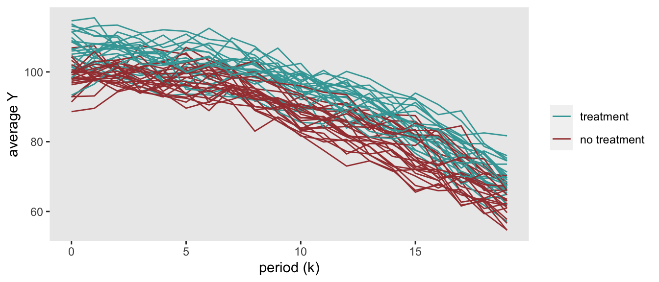
The simulated data will include 48 clusters over 20 time periods. 24 will be randomized to the control arm, 24 to the intervention. For each cluster and period, there are 30 individuals. The figure shows the cluster averages at each time point for one randomly generated data set:

The data generation process that underlies this plot is:
is the outcome measurement for individual in cluster at period . In this case, . There is an increasing decline in over time (based on the quadratic term ). is a treatment indicator for cluster , and , and the treatment effect is .
is a cluster-level random intercept for cluster , . is a cluster-specific time period effect for each time period ; the vector of cluster-time effects , where is a covariance matrix based on a diagonal matrix and an auto-regressive correlation structure :
and
The simstudy definitions establish , , , and . The vector is created separately in the actual data generation process using addCorGen, using and . Here are the initial definitions:
def <- defData(varname = "b0", formula = 0, variance = 6)
def <- defData(def, varname = "A", formula = "1;1", dist = "trtAssign")
def <- defData(def, varname = "mu", formula = 0, dist = "nonrandom")
def <- defData(def, varname = "s2", formula = 16, dist = "nonrandom")

defOut <- defDataAdd(varname = "y",
  formula = "100 + b0 + b1k - 0.1 * k^2 + 5*A",
  variance = 9)
I’ve wrapped the data generation process inside a function so that I can use it in a replication study at the end of the post. The function adds a normalized version of time and ensures that the site variable is a factor, both adjustments needed for modeling.
s_generate <- function() {

  d <- genData(48, def, id = "site")
  d <- addPeriods(d, 20, "site", perName = "k")

  d <- addCorGen(dtOld = d, idvar = "site", nvars = 20,
                 rho = .7, corstr = "ar1",
                 dist = "normal", param1 = "mu", param2 = "s2", cnames = "b1k")

  d <- genCluster(d, "timeID", numIndsVar = 30, level1ID = "id")
  d <- addColumns(defOut, d)

  d[, normk := (k - min(k))/(max(k) - min(k))]
  d[, site := as.factor(site)]

  d[]
}

set.seed(123)
dd <- s_generate()
Some modeling options
If we are interested in accounting for the secular (or time) trend when estimating the treatment effect, we have a number of different options. We can assume there is no structure to the pattern of time, we can impose an extreme form of structure, or we can try to find a flexible middle ground.
Time without structure
In stepped wedge designs - it is quite common to assume little if no structure in time trends. In the context of a CRT this could be set up by including a time-specific effect for each period , as in this model for an outcome for individual in group :
where is an indicator for treatment , and is set to 1 if cluster has been randomized to the intervention. and are the intercept and random intercept, respectively. is the effect size parameter. is the time-specific effect for period . This is a totally reasonable approach to take, but if starts to get quite large, we would need to need estimate large number of parameters ( period parameters, to be more precise), which is not always desirable, so we won’t take this approach here.
Time with over-simplified structure
An alternative approach is to model time in a linear fashion as
where we have a single parameter instead of period parameters. Here is an estimate of the treatment effect using a mixed effects model assuming a common linear time trend:
linear <- lmer(y ~ A + k + ( 1  | site) , data = dd)
summary(linear)$coefficients["A", c("Estimate", "Std. Error")]
## Estimate Std. Error
## 6.533 0.844The linear model gets around the problem of a large number parameters, but it imposes a very strong assumption that the outcome changes linearly over time (and in this case at the same rate for each cluster). This is unlikely to be the case. We could fit a quadratic model like
but the assumption is still quite strong. We could also fit a mixed effects model with a random slope as well:
But, if the temporal trend is not linear, there is no reason to think this would be the best approach.
Mixed effects model with fixed cubic spline and random intercept
We can introduce some flexibility into the model by using a cubic spline, which is constructed using a piece-wise cubic polynomial defined by specific points (knots) along the x-axis.
The cubic spline model is fit in R using the function bs in the splines package. In order to get more stable estimates, I’ve standardized the time measurement before using it in the model. In this case, the effect size estimate and standard error are the same as the linear model.
fix_cs <- lmer(y ~ A + bs(normk) + ( 1  | site) , data = dd)
summary(fix_cs)$coefficients["A", c("Estimate", "Std. Error")]
## Estimate Std. Error
## 6.533 0.844Mixed effects model with random cubic spline
There is no reason to believe that each cluster shares the same time trend, as assumed in the first two models estimated here. So now we introduce additional flexibility by fitting random cubic spline for each cluster.
The only difference between the fixed cubic spline model estimation is that the bs function appears in random effect portion of the model. The effect size estimate is slightly more biased than the previous estimates but has slightly less uncertainty.
ran_cs <- lmer(y ~ A + ( bs(normk) | site) , data = dd)## Warning in checkConv(attr(opt, "derivs"), opt$par, ctrl = control$checkConv, :
## Model failed to converge with max|grad| = 0.00672918 (tol = 0.002, component 1)summary(ran_cs)$coefficients["A", c("Estimate", "Std. Error")]## Estimate Std. Error
## 6.56 0.80Generalized additive model with site-specific smoothing
Another flexible modeling approach is the generalized additive model, which provides potentially even more flexibility than the spline models and can provide protections against over fitting. The underlying flexibility of the GAM is due to the wide range of basis functions that are available for the construction of the curve. I recommend taking a look the link for a nice introduction.
In this case, the model includes cluster-specific curves :
We estimate the model using the gamm function in the mgcv package. By setting the bs argument to “fs” in the smoothing function s, we will get estimated cluster-specific curves. “fs” refers to a special smooth factor interaction basis, where the interaction in this case is between site and time .
gam <- gamm(y ~ A + s(k, site, bs = "fs", k = 5), data = dd, method="REML")
cbind(summary(gam$gam)$p.coeff, summary(gam$gam)$se)[2,]
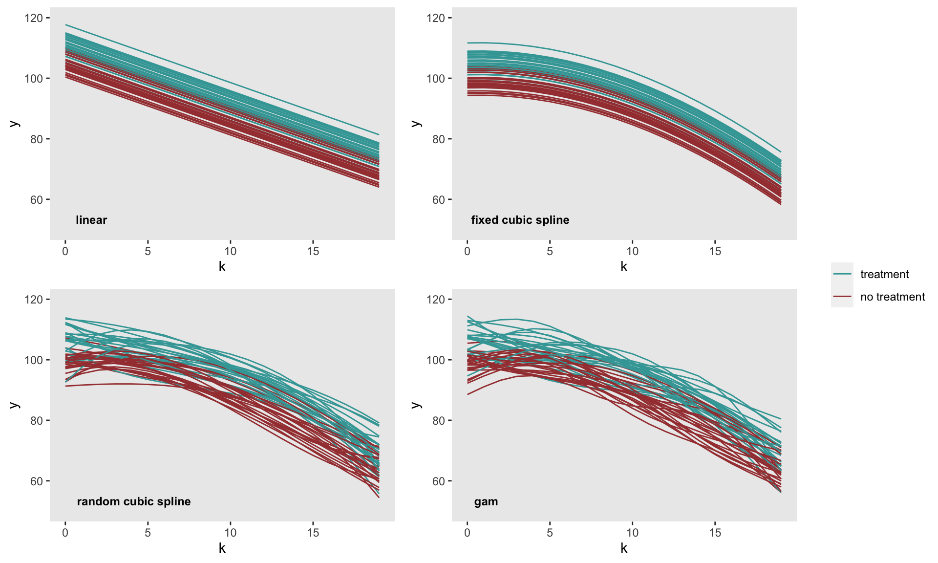
## [1] 6.537 0.846The figure below shows the predicted site-specific curves for each of the estimated models. The rigidity of the linear and fixed cubic spline models is pretty clear. And in at least this particular case, the two flexible methods appear to generate quite similar predicted curves.

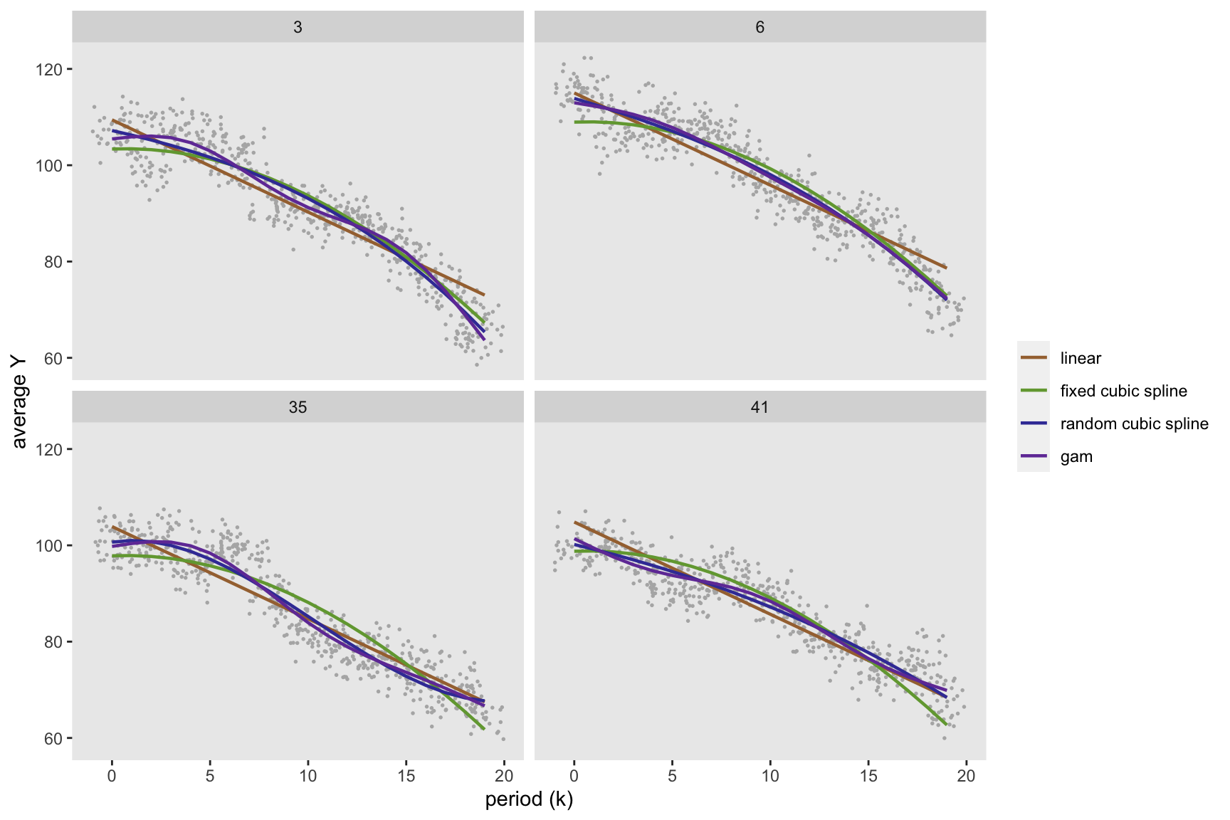
The next figure shows the individual-level outcomes and the predicted curves for a small number of sites. It is clear that the curves for the less flexible methods are biased. The similarity of the flexible models is particularly evident here.

Evaluating bias and variance of treatment effect estimate
The results from a single data set are interesting, but we really need to understand how well the models perform over a large number of data sets. How do the model estimates of the true treatment effect () compare when considering bias, variance, and coverage of the 95% confidence interval?
The replication process requires generating data and then fitting the models. The data generation uses the data definitions and data generating function provided earlier in the post. In this case, we will use 1000 data sets.
replicate <- function(){

  dd <- s_generate()

  linear <- lmer(y ~ A + k + ( 1  | site) , data = dd)
  est.lin <- summary(linear)$coefficients["A", c("Estimate", "Std. Error")]

  fix_cs <- lmer(y ~ A + bs(normk) + ( 1  | site) , data = dd)
  est.fcs <- summary(fix_cs)$coefficients["A", c("Estimate", "Std. Error")]

  ran_cs <- lmer(y ~ A + ( bs(normk) | site) , data = dd)
  est.rcs <- summary(ran_cs)$coefficients["A", c("Estimate", "Std. Error")]

  gam <- gamm(y ~ A + s(k, site, bs = "fs", k = 5), data = dd, method="REML")
  est.gam <- cbind(summary(gam$gam)$p.coeff, summary(gam$gam)$se)[2,]

  dres <- data.table(t(est.lin), t(est.fcs), t(est.rcs), t(est.gam))
  setnames(dres,
    c("d.lin", "se.lin", "d.fcs", "se.fcs", "d.rcs", "se.rcs", "d.gam", "se.gam")
  )

  dres[]
}

res <- rbindlist(pblapply(1:1000, function(x) replicate()))
Each replication provides the point estimate of the treatment effect as well as the estimate of the standard error. Here is a sampling of the results:
res## d.lin se.lin d.fcs se.fcs d.rcs se.rcs d.gam se.gam
## 1: 4.53 0.847 4.53 0.847 4.73 0.805 4.55 0.850
## 2: 3.68 0.911 3.68 0.911 3.68 0.873 3.77 0.908
## 3: 3.34 0.734 3.34 0.734 3.33 0.685 3.36 0.729
## 4: 4.95 0.690 4.95 0.690 5.07 0.680 4.89 0.688
## 5: 5.75 0.865 5.75 0.865 5.67 0.776 5.81 0.868
## ---
## 996: 5.27 1.001 5.27 1.001 5.17 0.974 5.35 1.008
## 997: 5.94 0.842 5.94 0.842 6.10 0.818 5.89 0.839
## 998: 4.92 0.910 4.92 0.910 4.91 0.876 4.94 0.916
## 999: 4.72 0.799 4.72 0.799 4.41 0.696 4.71 0.786
## 1000: 4.56 0.887 4.56 0.887 4.74 0.852 4.54 0.888The average of the point estimates across all replications provides an estimate of the bias for each model. The four approaches are relatively unbiased, and this includes the less flexible approaches that didn’t seem to do so well at prediction on the individual level. The random cubic spline seems to have slightly less bias:
res[, .(lin = mean(d.lin), fcs = mean(d.fcs), rcs = mean(d.rcs), gam = mean(d.gam))] - 5## lin fcs rcs gam
## 1: 0.0314 0.0314 0.0206 0.0304A comparison of the observed standard errors suggests that the random cubic spline model is slightly more variable than the other three modeling approaches, suggesting a bias-variance trade-off.
res[, .(lin = sd(d.lin), fcs = sd(d.fcs), rcs = sd(d.rcs), gam = sd(d.gam))]## lin fcs rcs gam
## 1: 0.92 0.92 0.941 0.919And while all four methods underestimate the uncertainty, on average, the random cubic spline model most severely underestimated the standard errors:
res[, .(lin = mean(se.lin), fcs = mean(se.fcs), rcs = mean(se.rcs), gam = mean(se.gam))]## lin fcs rcs gam
## 1: 0.907 0.907 0.87 0.908Consistent with the disparities in variance estimates, the random cubic splines did not perform as well with respect to the coverage rates of the 95% confidence intervals:
coverage <- function(est, se) {
  rmin <- est - 1.96 * se
  rmax <- est + 1.96 * se

  mean(rmin < 5 & rmax > 5)
}

res[, .(lin = coverage(d.lin, se.lin), fcs = coverage(d.fcs, se.fcs),
        rcs = coverage(d.rcs, se.rcs), gam = coverage(d.gam, se.gam))]
## lin fcs rcs gam
## 1: 0.944 0.944 0.924 0.94It will be interesting to see how the bias-variance trade-off plays out in the context of a stepped wedge design, particularly if the outcomes are binary. Will the less flexible methods continue to perform as well as the GAM model, and will the cubic spline model continue to underestimate the standard errors? More to come. (The next post is now available.)