Really, the only problem with the simstudy package (😄) is that there is a hard limit to the possible probability distributions that are available (the current count is 15 - see here for a complete description). However, it turns out that there is more flexibility than first meets the eye, and we can easily accommodate a limitless number as long as you are willing to provide some extra code.
I am going to illustrate this with two examples, first by implementing a truncated normal distribution, and second by implementing the flexible non-linear data generating algorithm that I described last time.
Before we get going, here are the necessary libraries:
library(simstudy)
library(data.table)
library(msm)
library(ggplot2)
library(mgcv)
General concept
In the data definition step, it is possible to specify any valid R function in the formula argument. If dist is specified as “nonrandom”, then simstudy will generate data based on that function. (Yes, the specification as “nonrandom” is a bit awkward since we are defining a stochastic data generating process in this case; in future versions I plan to allow dist to be specified as “custom” to make this less dissonant.)
In this example, I want to be able to generate data from a truncated normal distribution. There is an existing function rtnorm in the msm package that I can take advantage here. What I have done is essentially create a wrapper function that makes a single draw from the truncated distribution with a specified mean, standard deviation, and pair of truncation bounds:
trunc_norm <- function(mean, sd, lower, upper) {
  rtnorm(n = 1, mean = mean, sd = sd, lower = lower, upper = upper)
}
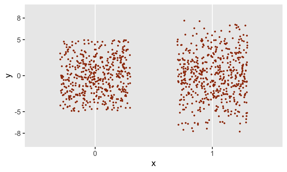
Now that trunc_norm has been created, I am free to use this is in a data definition statement. And even more important, the call to trunc_norm can depend on other variables; in this case, I have created binary variable x that will determine the upper and lower bounds of the distribution. When \(x=0\), the \(N(0, 3.5^2)\) distribution is truncated at -5 and 5, and when \(x=1\), the distribution is truncated at -8 and 8.
defI <- defData(varname = "x", formula = 0.5, dist = "binary")
defI <- defData(defI, varname = "y",
  formula = "trunc_norm(mean = 0, sd = 3.5,
               lower = -5 + -3*x, upper = 5 + 3*x)",
  dist = "nonrandom")
The generated data appear to have the properties that we would expect:
dd <- genData(1000, defI)
Application to non-linear data generation
Last time, I described an approach to generate a variable \(y\) that has a non-linear response with respect to an input variable \(x\). At the end of that post, I created two functions, one of which can be referred to in the defData statement to generate the data. (I plan on implementing these functions in simstudy, but I was eager to get the concept out there in case any one has some suggestions or could use this feature right away.)
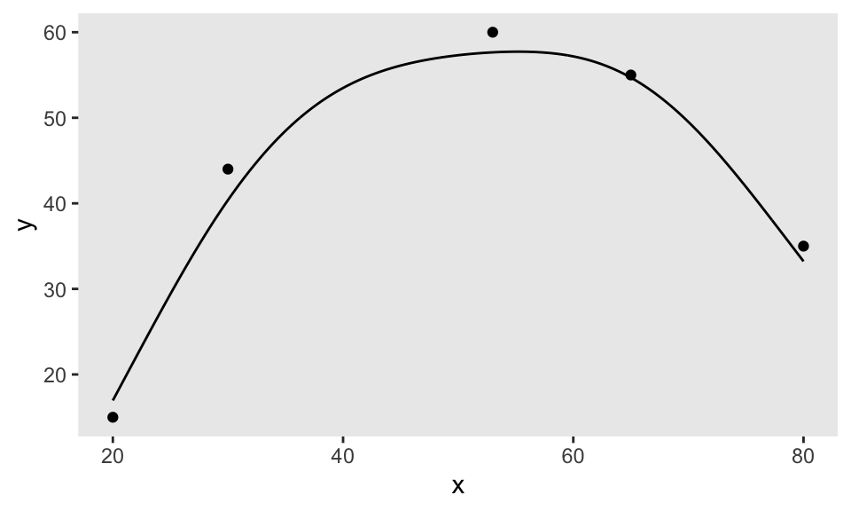
In the first step, I need to generate a smooth function by specifying a few points. I do this by calling getNLfunction. (If you want the code for this, let me know, but I actually provided most of it last week.) The variable nlf is an object that contains the function:
dpoints <- data.table(x = c(20, 30, 53, 65, 80), y = c(15, 44, 60, 55, 35))
nlf <- getNLfunction(dpoints)
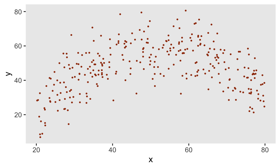
The function genNL makes predictions based on the nlf object and adds a little Gaussian noise. We use the same approach as we did above for the truncated normal to generate different responses \(y\) based on the level of \(x\):
def <- defData(varname = "x", formula = "20;80", dist = "uniform")
def <- defData(def, varname = "y",
  formula = "genNL(nf = ..nlf, x, sd = 10)", dist = "nonrandom")

dd <- genData(300, def)
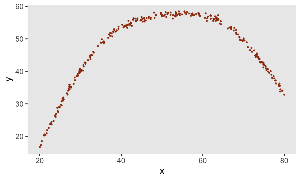
And if we introduce much less noise, we get much closer to the original underlying function specified by our points:
def <- defData(varname = "x", formula = "20;80", dist = "uniform")
def <- defData(def, varname = "y",
  formula = "genNL(nf = ..nlf, x, sd = 0.5)", dist = "nonrandom")

dd <- genData(300, def)