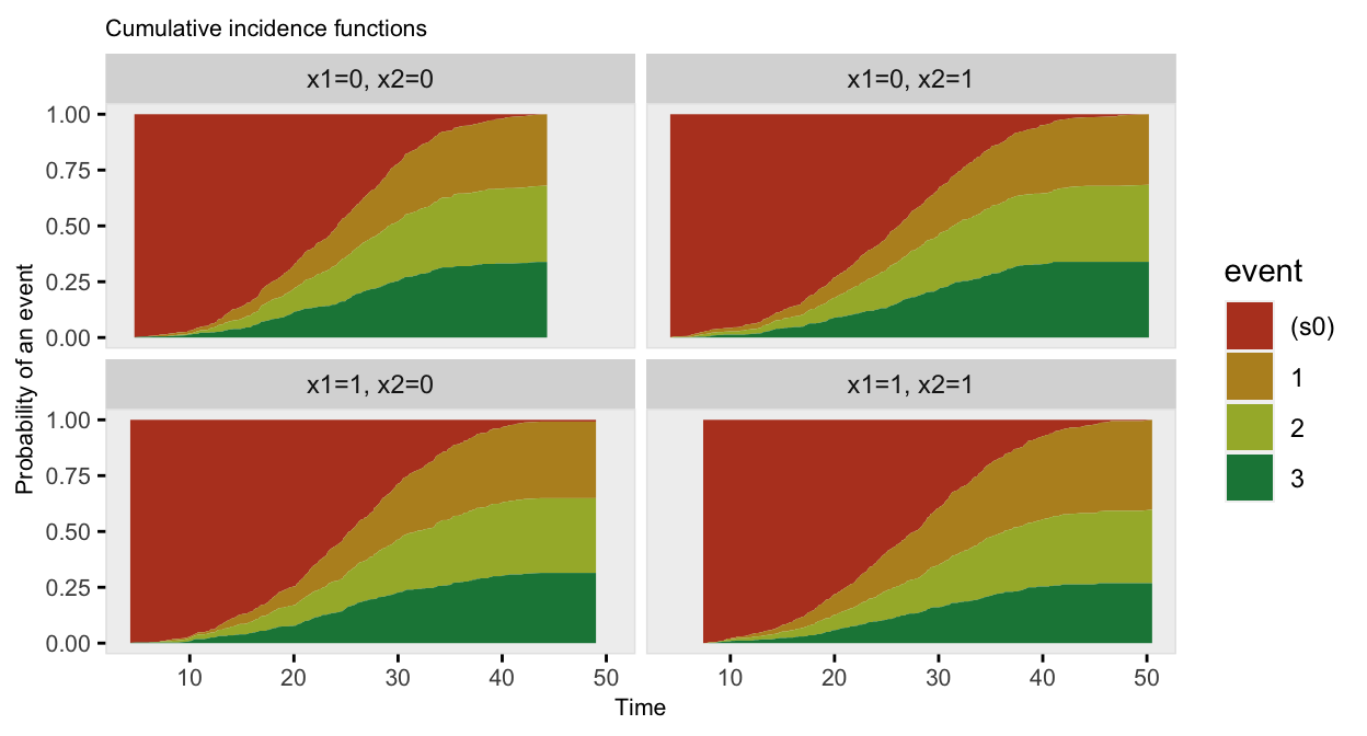
Adding competing risks in survival data generation

I am working on an update of simstudy that will make generating survival/time-to-event data a bit more flexible. There are two biggish enhancements. The first facilitates generation of competing events, and the second allows for the possibility of generating survival data that has time-dependent hazard ratios. This post focuses on the first enhancement, and a follow up will provide examples of the second. (If you want to try this at home, you will need the development version of simstudy, which you can install using devtools::install_github(“kgoldfeld/simstudy”).)

Competing risks

In standard survival analysis, we are interested in understanding the distribution of time to a single event, such as time to death or time to symptom-free recovery. However, there may be situations where two there are at least two possible events, and the occurrence of one precludes the occurrence of the other. In this case, we say that the events are competing risks. In the work that motivated this simstudy enhancement, we are trying to model the time to opioid overdose death for people being released from jail, but there are at least two other competing risks, death from other causes and re-incarceration. In addition, there is censoring, which from a data generation point of view (though maybe not from an analytic perspective), can also be considered a competing risk.

Generating competing risk outcomes under 0.4.0

Previously, it was possible to generate competing risk outcomes, but it had to be done “manually” with additional lines of code or data definitions. It was a bit cumbersome:

library(simstudy)
library(data.table)
library(survival)

First, we would generate a data set with genSurv:

d1 <- defData(varname = "x1", formula = .5, dist = "binary")
d1 <- defData(d1, "x2", .5, dist = "binary")

dS <- defSurv(varname = "event_1", formula = "-12 - 0.1*x1 - 0.2*x2", shape = 0.3)
dS <- defSurv(dS, "event_2", "-12 - 0.3*x1 - 0.2*x2", shape = 0.3)
dS <- defSurv(dS, "event_3", "-12 - 0.4*x1 - 0.3*x2", shape = 0.3)
dS <- defSurv(dS, "censor", "-13", shape = 0.3)

set.seed(2140)

dtCov <- genData(3001, d1)
dtSurv <- genSurv(dtCov, dS)

head(dtSurv)

##    id x1 x2 censor event_1 event_2 event_3
## 1:  1  0  1 56.809  40.321  35.050  48.356
## 2:  2  0  0 62.278  24.865  23.121  19.198
## 3:  3  1  0 25.650  27.898  24.716  49.633
## 4:  4  1  1 51.486  35.065  44.731  40.086
## 5:  5  1  0 54.522  37.042  49.701  34.751
## 6:  6  1  0 42.749  41.419  34.136  43.811

And then we would add the observed time variable with a new data definition and call to addColumns:

f <- "(time==censor)*0 + (time==event_1)*1 + (time==event_2)*2 + (time==event_3)*3"

cdef <- defDataAdd(varname = "time", 
  formula = "pmin(censor, event_1, event_2, event_3)", dist = "nonrandom")
cdef <- defDataAdd(cdef, varname = "event", 
  formula = f, 
  dist = "nonrandom")

dtSurv_final <- addColumns(cdef, dtSurv)
head(dtSurv_final)

##    id x1 x2 censor event_1 event_2 event_3   time event
## 1:  1  0  1 56.809  40.321  35.050  48.356 35.050     2
## 2:  2  0  0 62.278  24.865  23.121  19.198 19.198     3
## 3:  3  1  0 25.650  27.898  24.716  49.633 24.716     2
## 4:  4  1  1 51.486  35.065  44.731  40.086 35.065     1
## 5:  5  1  0 54.522  37.042  49.701  34.751 34.751     3
## 6:  6  1  0 42.749  41.419  34.136  43.811 34.136     2

Streamlined approach

The function addCompRisk can now generate an observed time variable (which will be the first of the four event times). This is done by specifying a timeName argument that will represent the observed time value. The event status is indicated in the field set by the eventName argument (which defaults to “event”). And, if a variable name is indicated in the censorName argument, the censored events automatically have a value of 0.

dtSurv_final <- addCompRisk(dtSurv, 
  events = c("event_1", "event_2", "event_3", "censor"), 
  timeName = "time", censorName = "censor")

head(dtSurv_final)

##    id x1 x2   time event    type
## 1:  1  0  1 35.050     2 event_2
## 2:  2  0  0 19.198     3 event_3
## 3:  3  1  0 24.716     2 event_2
## 4:  4  1  1 35.065     1 event_1
## 5:  5  1  0 34.751     3 event_3
## 6:  6  1  0 34.136     2 event_2

The competing risk data can be plotted using the cumulative incidence functions (rather than the survival curves):

The data generation can be streamlined even further, as there is no need to call addCompRisk at all. The same arguments can be provided directly in the call to genSurv, so everything is done at once. And there is no need to explicitly name the events, as they are extracted from the survival distribution definitions:

dtSurv_final <- genSurv(dtCov, dS, timeName = "time", censorName = "censor")
head(dtSurv_final)

##    id x1 x2   time event    type
## 1:  1  0  1 30.229     3 event_3
## 2:  2  0  0 28.473     1 event_1
## 3:  3  1  0 11.654     0  censor
## 4:  4  1  1 28.248     1 event_1
## 5:  5  1  0 28.524     3 event_3
## 6:  6  1  0 18.255     0  censor

If you don’t want to generate competing risk data, and you can set timeName to NULL, or just not specify it:

dtSurv_final <- genSurv(dtCov, dS)
head(dtSurv_final)

##    id x1 x2 censor event_1 event_2 event_3
## 1:  1  0  1 40.276  16.858  42.624  34.609
## 2:  2  0  0 69.382  24.191  37.574  10.783
## 3:  3  1  0 26.637  48.476  54.240  60.507
## 4:  4  1  1 36.697  46.690  36.443  43.195
## 5:  5  1  0 64.498  36.755  39.666  10.935
## 6:  6  1  0 69.150  38.706  44.930  17.668

R survival analysis