simstudy update: ordinal data generation that violates proportionality

genOrdCat

The way to generate ordered categorical data in simstudy is with the function genOrdCat. The probability of responses or categories is specified for the reference group - in this case the unexposed. The effect of exposure (and any other covariates) is expressed in an adjustment variable (here z). In the data generating process defined below, we are saying that the cumulative odds for the exposed is about 1/2 the odds for the unexposed at each level of response x. This is the proportional odds assumption, and on the log(OR) scale this is \(log(0.5) = -0.7\).

baseprobs <- c(0.35, 0.25, 0.20, 0.20)

defA <- defData(varname = "exposed", formula = "1;1", dist = "trtAssign")
defA <- defData(defA, varname = "z", formula = "-0.7 * exposed", dist = "nonrandom")

set.seed(230)

dd <- genData(25000, defA)
dx <- genOrdCat(dd, adjVar = "z", baseprobs, catVar = "response")

Here is a manual calculation of the observed probabilities and odds (for a more visual interpretation of all of this, see this description):

dp <- dx[, .(n = .N), keyby = .(exposed, response)]
dp[, p := n/sum(n), keyby = .(exposed)]
dp[, cump := round(cumsum(p),3), keyby = .(exposed)]
dp[, codds := (1-cump)/cump]
dp[, lcodds := log(codds)]
dp

##    exposed response    n    p cump codds lcodds
## 1:       0        1 4406 0.35 0.35  1.84   0.61
## 2:       0        2 3168 0.25 0.61  0.65  -0.43
## 3:       0        3 2471 0.20 0.80  0.24  -1.41
## 4:       0        4 2455 0.20 1.00  0.00   -Inf
## 5:       1        1 6616 0.53 0.53  0.89  -0.12
## 6:       1        2 2860 0.23 0.76  0.32  -1.14
## 7:       1        3 1638 0.13 0.89  0.12  -2.08
## 8:       1        4 1386 0.11 1.00  0.00   -Inf

We can calculate the cumulative odds ratio at each response level …

dc <- dcast(dp, response ~ exposed, value.var = "codds")
dc [, cOR := `1`/`0`]
dc

##    response    0    1  cOR
## 1:        1 1.84 0.89 0.48
## 2:        2 0.65 0.32 0.49
## 3:        3 0.24 0.12 0.51
## 4:        4 0.00 0.00  NaN

and the log(cOR):

dc <- dcast(dp, response ~ exposed, value.var = "lcodds")
dc [, lcOR := `1` - `0`]
dc

##    response     0     1  lcOR
## 1:        1  0.61 -0.12 -0.73
## 2:        2 -0.43 -1.14 -0.71
## 3:        3 -1.41 -2.08 -0.67
## 4:        4  -Inf  -Inf   NaN

Estimating the parameters of the model using function clm in the ordinal package, we can recover the original parameters quite well. Note that the threshold coefficients are log cumulative odds at each response level for the reference group, the unexposed.

library(ordinal)
clmFit <- clm(response ~ exposed, data = dx)
summary(clmFit)

## formula: response ~ exposed
## data:    dx
## 
##  link  threshold nobs  logLik    AIC      niter max.grad cond.H 
##  logit flexible  25000 -31750.20 63508.39 4(0)  6.05e-07 1.9e+01
## 
## Coefficients:
##         Estimate Std. Error z value Pr(>|z|)    
## exposed  -0.7146     0.0236   -30.3   <2e-16 ***
## ---
## Signif. codes:  0 '***' 0.001 '**' 0.01 '*' 0.05 '.' 0.1 ' ' 1
## 
## Threshold coefficients:
##     Estimate Std. Error z value
## 1|2  -0.6017     0.0176   -34.3
## 2|3   0.4305     0.0173    24.9
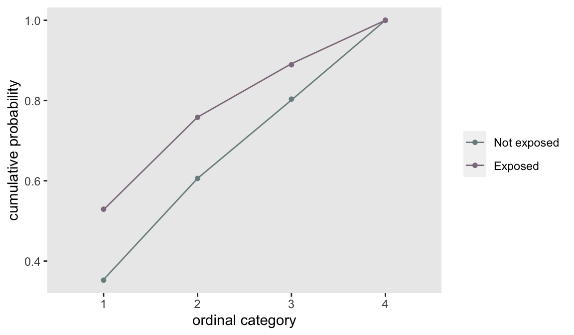
## 3|4   1.3941     0.0201    69.3

A plot of the modeled cumulative probabilities (the lines) shows that the proportionality assumption fit the observed data (the points) quite well.

Non-proportional odds

With the recent update, it is now possible to generate data that violate the proportionality assumption by using new arguments npVar and npAdj. npVar indicates the variable(s) for which the non-proportional assumption is violated, and npAdj is a vector that specifies the extent and direction of the violation at each level of the response (on the logit scale). (Since the log odds ratio for the highest level response is infinite, the final value in the vector has no impact.)

dx <- genOrdCat(dd, baseprobs = baseprobs, catVar = "response", adjVar = "z",
                npVar = "exposed", npAdj = c(1.0, 0, -1.0, 0))

dp <- dx[, .(n = .N), keyby = .(exposed, response)]
dp[, p := n/sum(n), keyby = .(exposed)]
dp[, cump := round(cumsum(p),3), keyby = .(exposed)]
dp[, codds := (1-cump)/cump]
dp[, lcodds := log(codds)]
dp

##    exposed response    n     p cump codds lcodds
## 1:       0        1 4351 0.348 0.35 1.874   0.63
## 2:       0        2 3145 0.252 0.60 0.667  -0.41
## 3:       0        3 2444 0.196 0.80 0.258  -1.36
## 4:       0        4 2560 0.205 1.00 0.000   -Inf
## 5:       1        1 3506 0.280 0.28 2.571   0.94
## 6:       1        2 5784 0.463 0.74 0.346  -1.06
## 7:       1        3 2629 0.210 0.95 0.048  -3.03
## 8:       1        4  581 0.046 1.00 0.000   -Inf

We can see that the cumulative OR for response level 2 remains close to 0.5, but the cORs shift away from 0.5 response levels 1 and 3.

dc <- dcast(dp, response ~ exposed, value.var = "codds")
dc [, cOR := `1`/`0`]
dc

##    response    0     1  cOR
## 1:        1 1.87 2.571 1.37
## 2:        2 0.67 0.346 0.52
## 3:        3 0.26 0.048 0.19
## 4:        4 0.00 0.000  NaN

On the log odds scale, it is possible to see the direct effect of the values specified in the adjustment vector npAdj. The observed log cumulative OR at response level 1 is \(1.0 - 0.7 = 0.3\), and the at level 3 it is \(-1.0 - 0.7 = -1.7:\)

dc <- dcast(dp, response ~ exposed, value.var = "lcodds")
dc [, lcOR := `1` - `0`]
dc

##    response     0     1  lcOR
## 1:        1  0.63  0.94  0.32
## 2:        2 -0.41 -1.06 -0.66
## 3:        3 -1.36 -3.03 -1.68
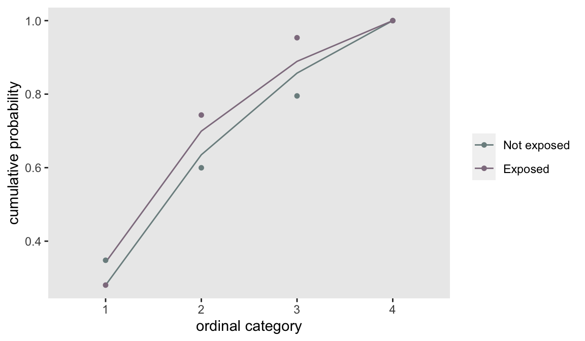
## 4:        4  -Inf  -Inf   NaN

The lack of proportionality is confirmed by a plot of the model fit with a proportional odds assumption along with the observed cumulative proportions. Since the model imposes proportionality, the observed points no longer lie along the prediction line: