simstudy update: adding flexibility to data generation

A new version of simstudy (0.3.0) is now available on CRAN and on the package website. Along with some less exciting bug fixes, we have added capabilities to a few existing features: double-dot variable reference, treatment assignment, and categorical data definition. These simple additions should make the data generation process a little smoother and more flexible.

Using non-scalar double-dot variable reference

Double-dot notation was introduced in the last version of simstudy to allow data definitions to be more dynamic. Previously, the double-dot variable could only be a scalar value, and with the current version, double-dot notation is now also array-friendly.

Before the examples, here are the necessary packages for this post:

library(simstudy)
library(data.table)
library(ggplot2)

Example 1

In the first example, we want to create a mixture distribution from a vector of values (which we can also do using a categorical distribution, more on that in a little bit). We can define the mixture formula in terms of the vector. In this case we are generating permuted block sizes of 2 and 4, specified as

sizes <- c(2, 4)

The data definition references each element of the vector:

defblk <- defData(varname = "blksize", 
   formula = "..sizes[1] | .5 + ..sizes[2] | .5", dist = "mixture")

genData(1000, defblk)

##         id blksize
##    1:    1       2
##    2:    2       4
##    3:    3       2
##    4:    4       4
##    5:    5       4
##   ---             
##  996:  996       4
##  997:  997       4
##  998:  998       4
##  999:  999       4
## 1000: 1000       4

Example 2

In this second example, there is a vector variable tau of positive real numbers that sum to 1, and we want to calculate the weighted average of three numbers using tau as the weights. We could use the following code to estimate a weighted average theta:

tau <- rgamma(3, 5, 2)
tau <- tau / sum(tau)
tau

## [1] 0.362 0.400 0.238

d <- defData(varname = "a", formula = 3, variance = 4)
d <- defData(d, varname = "b", formula = 8, variance = 2)
d <- defData(d, varname = "c", formula = 11, variance = 6)
d <- defData(d, varname = "theta", formula = "..tau[1]*a + ..tau[2]*b + ..tau[3]*c", 
  dist = "nonrandom")

set.seed(19483)
genData(4, d)

##    id    a    b     c theta
## 1:  1 1.87 8.16 13.72  7.21
## 2:  2 3.45 7.45  6.08  5.68
## 3:  3 7.41 6.27 10.21  7.62
## 4:  4 2.34 9.52 10.01  7.04

However, we can simplify the calculation of theta a bit by using matrix multiplication:

d <- updateDef(d, changevar = "theta", newformula = "t(..tau) %*% c(a, b, c)")

set.seed(19483)
genData(4, d)

##    id    a    b     c theta
## 1:  1 1.87 8.16 13.72  7.21
## 2:  2 3.45 7.45  6.08  5.68
## 3:  3 7.41 6.27 10.21  7.62
## 4:  4 2.34 9.52 10.01  7.04

Example 3

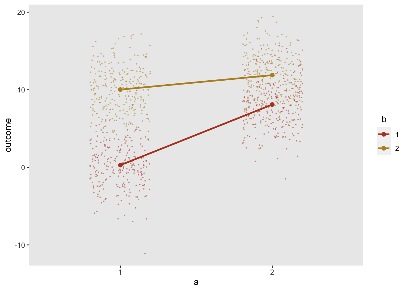
The arrays can also have multiple dimensions, as in a \(m \times n\) matrix. If we want to specify the mean outcomes for a \(2 \times 2\) factorial study design with two interventions \(a\) and \(b\), we can use a simple matrix and draw the means directly from the matrix, which in this example is stored in the variable effect:

effect <- matrix(c(0, 8, 10, 12), nrow = 2)
effect

##      [,1] [,2]
## [1,]    0   10
## [2,]    8   12

Using double dot notation, it is possible to reference the matrix cell values directly, depending on the values of a and b:

d1 <- defData(varname = "a", formula = ".5;.5", variance = "1;2", dist = "categorical")
d1 <- defData(d1, varname = "b", formula = ".5;.5", 
              variance = "1;2", dist = "categorical")
d1 <- defData(d1, varname = "outcome", formula = "..effect[a, b]",
              variance = 9, dist="normal")

dx <- genData(1000, d1)
dx

##         id a b outcome
##    1:    1 1 2   12.07
##    2:    2 2 2    9.70
##    3:    3 2 2   10.76
##    4:    4 2 2   11.04
##    5:    5 2 1    5.51
##   ---                 
##  996:  996 1 1   -2.80
##  997:  997 2 1    5.15
##  998:  998 2 2   19.47
##  999:  999 2 1   10.53
## 1000: 1000 2 1    3.89

The plot shows individual values as well as mean values by intervention arm:

Assigned treatment using trtAssign distribution in `defData`

The function trtAssign currently provides functionality to randomize group assignments using stratification and non-standard ratios (e.g. 2:2:1 for a three arm trial). Starting with version 0.3.0, it is also possible to generate these treatment assignments directly in the defData and genData process without a separate call to trtAssign. We’ve done this by adding trtAssign as a possible distribution.

In this example, randomization is stratified by gender and age (specified in the variance argument), and randomization is 1:1 treatment to control (specified in formula). The outcome y is effected by both of these factors as well as the treatment assignment variable rx.

def <- defData(varname = "male", dist = "binary", 
               formula = .5 , id="cid")
def <- defData(def, varname = "over65", dist = "binary",  
               formula = "-1.7 + .8*male", link="logit")
def <- defData(def, varname = "rx", dist = "trtAssign",
               formula = "1;1", variance = "male;over65")
def <- defData(def, varname = "y", dist = "normal", 
               formula = "20 + 5*male + 10*over65 + 10*rx", variance = 40)

dtstudy <- genData(330, def)
dtstudy

##      cid male over65 rx    y
##   1:   1    1      0  0 20.4
##   2:   2    1      0  0 23.9
##   3:   3    0      1  0 23.7
##   4:   4    1      0  1 25.9
##   5:   5    0      1  0 35.4
##  ---                        
## 326: 326    1      1  1 46.3
## 327: 327    1      0  1 33.2
## 328: 328    1      0  1 35.5
## 329: 329    1      1  0 42.2
## 330: 330    0      0  0 12.5

Here are the counts and average outcomes for each gender, age, and treatment combination:

dtstudy[, .(n = .N, avg = round(mean(y), 1)), keyby = .(male, over65, rx)]

##    male over65 rx  n  avg
## 1:    0      0  0 72 20.3
## 2:    0      0  1 72 30.3
## 3:    0      1  0 12 28.7
## 4:    0      1  1 12 38.5
## 5:    1      0  0 55 25.0
## 6:    1      0  1 56 34.3
## 7:    1      1  0 26 36.6
## 8:    1      1  1 25 45.7

Categogorical data

Finally, in previous versions, the categorical distribution generated a set of integer categories:

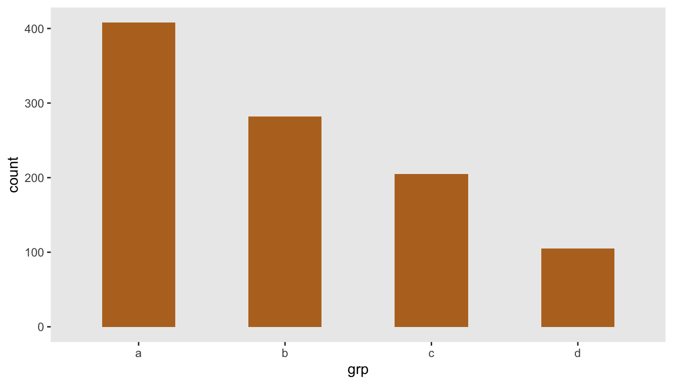
def <- defData(varname = "grp", formula = ".4;.3;.2;.1", dist="categorical")
genData(1000, def)

##         id grp
##    1:    1   1
##    2:    2   4
##    3:    3   4
##    4:    4   1
##    5:    5   2
##   ---         
##  996:  996   1
##  997:  997   4
##  998:  998   2
##  999:  999   4
## 1000: 1000   1

Now, it is possible to generate specific values or string categories by using the variance argument:

def <- defData(varname = "grp", formula = ".4;.3;.2;.1", 
               variance = "a;b;c;d", dist="categorical")

dd <- genData(1000, def)
dd

##         id grp
##    1:    1   d
##    2:    2   b
##    3:    3   a
##    4:    4   c
##    5:    5   b
##   ---         
##  996:  996   d
##  997:  997   a
##  998:  998   b
##  999:  999   a
## 1000: 1000   d

To replicate Example 1 above, here is an alternative way to generate block sizes of 2 and 4 using the categorical distribution and the new functionality.

defblk <- defData(varname = "blksize", 
   formula = ".5;.5", variance = "2;4", dist = "categorical")

genData(1000, defblk)

##         id blksize
##    1:    1       2
##    2:    2       4
##    3:    3       2
##    4:    4       4
##    5:    5       4
##   ---             
##  996:  996       2
##  997:  997       2
##  998:  998       2
##  999:  999       2
## 1000: 1000       2

Possible next steps

As we expand the functionality of simstudy, we realize that the current structure of the data definition table cannot always easily accommodate all of our new ideas. As a result, we have ended up having to shoehorn some solutions in non-intuitive ways as we grow. We are in the process of reconsidering that structure so that we won’t have (as many of) these awkward specifications in the future (though we will be making everything backwards compatible, so no worries there).

R simstudy