Sample size requirements for a Bayesian factorial study design

Setting the target

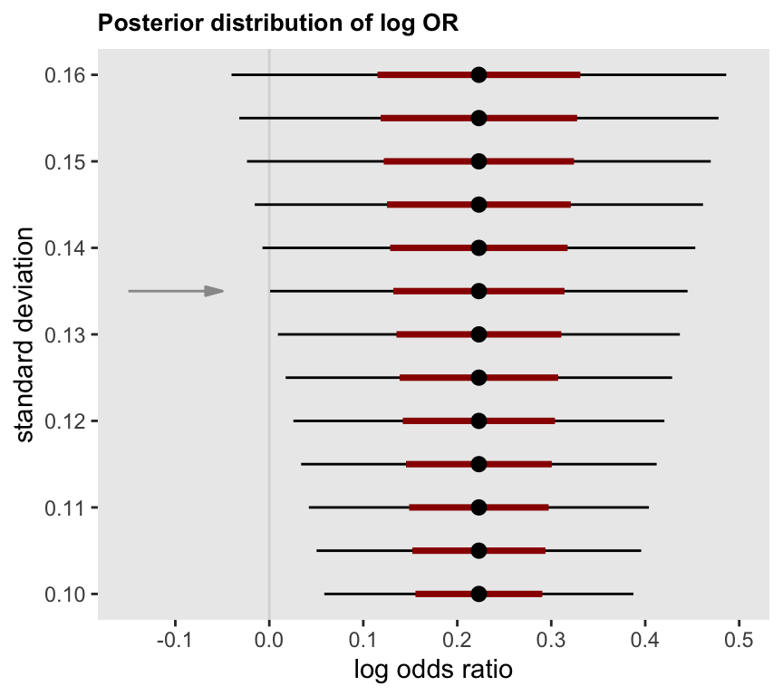
To determine the target level of precision, I assessed the width of the posterior distributions under different standard deviations. In particular, I identified the posterior probabilities with a mean OR = 1.25 \((log(OR) = 0.22)\) where \(P(log(OR) > 0) \ge 0.95\). The target OR is somewhat arbitrary, but seemed like a meaningful effect size based on discussions with my collaborators.

I did a quick search for the standard deviation that would yield a 95% threshold at or very close to 0. That is, 95% of the distribution should lie to the right of 0. Assuming that the target posterior distribution will be approximately normal with a mean of 0.22, I used the qnorm function to find the 95% thresholds for range of standard deviations between 0.10 and 0.15.

sd <- seq(.15, .10, by = -0.005)
cbind(sd, threshold = round(qnorm(.05, .22 , sd = sd), 3))

##          sd threshold
##  [1,] 0.150    -0.027
##  [2,] 0.145    -0.019
##  [3,] 0.140    -0.010
##  [4,] 0.135    -0.002
##  [5,] 0.130     0.006
##  [6,] 0.125     0.014
##  [7,] 0.120     0.023
##  [8,] 0.115     0.031
##  [9,] 0.110     0.039
## [10,] 0.105     0.047
## [11,] 0.100     0.056

It looks like the target standard deviation should be close to 0.135, which is also apparent from the plot of the 95% intervals centered at 0.22:

Using simulation to establish sample size

The final step was to repeatedly simulate data sets using different sample size assumptions, fitting models, and estimating the posterior distribution standard deviations for associated with each data set (and sample size). I evaluated sample sizes ranging from 400 to 650 individuals, increasing in increments of 50. For each sample size, I generated 250 data sets, for a total of 1,500 data sets and model estimates. Given that each model estimation is quite resource intensive, I generated all the data and estimated the models using a high performance computing environment that provided me with 90 nodes and 4 processors on each node so that the Bayesian MCMC process could all run in parallel - so parallelization of parallel processes. In total, this took about 2 hours to run.

(I am including the code in the addendum below. The structure is similar to what I have described in the past on how one might do these types of explorations with simulated data and Bayesian modelling.)

Below is the output for a single data set to provide an example of the data being generated by the simulations. We have estimated seven log-odds ratios (see here for an explanation of why there are seven), and the simulation returns a summary of the posterior distribution for each: selected quantiles and the standard deviation.

##      n    var p0.025 p0.25  p0.5 p0.75 p0.975    sd
## 1: 650 lOR[1]  0.113 0.269 0.354 0.441  0.603 0.126
## 2: 650 lOR[2]  0.410 0.569 0.652 0.735  0.892 0.123
## 3: 650 lOR[3]  0.427 0.585 0.667 0.752  0.906 0.123
## 4: 650 lOR[4]  0.367 0.526 0.608 0.691  0.851 0.122
## 5: 650 lOR[5]  0.436 0.592 0.675 0.757  0.913 0.122
## 6: 650 lOR[6]  0.703 0.861 0.945 1.028  1.180 0.122
## 7: 650 lOR[7]  0.722 0.886 0.969 1.054  1.214 0.125

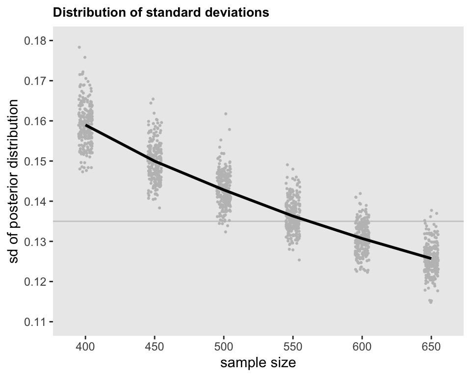
The plot below shows the estimated standard deviations for a single log-odds ratio (in this case \(\lambda_4\)), with a point for each of the 1,500 simulate data sets. At 550 subjects, the mean standard deviation (represented by the curve) is starting to get close to 0.135, but there is still quite a bit of uncertainty. To be safe, we might want to set the upper limit for the study to be 600 patients, because we are quite confident that the standard deviation will be low enough to meet our criteria (almost 90% of the standard deviations from the simulations were below 0.135, though at 650 patients that proportion was over 98%).

Addendum

This code generates repeated data sets under different sample size assumptions and draws samples from the posterior distribution for each of those data sets. The simulations are set up to run on a high performance computing (HPC) environment, so multiple data sets can be generated and analyzed simultaneously. If you do not have access to and HPC, you can run locally using lapply or mclapply rather than Slurm_lapply, but unless you have an extremely powerful desktop or laptop, expect these kinds of simulations to take days rather than hours.

One particularly interesting feature of the data generation process used in these simulations is that the effect size parameters are not considered to be fixed, but are themselves drawn from a distribution of parameters. Given that we are never certain about what the parameters should be in the data generation process, this adds an appropriate level of uncertainty that gets reflected in our target estimates. If we are slightly conservative in our sample size selection, this will take into account this additional uncertainty. Of course, how much uncertainty will depend on the situation.

library(cmdstanr)
library(simstudy)
library(data.table)
library(posterior)
library(slurmR)
library(glue)

s_define <- function() {
  
  f <- "..t_0 + ..t_a*a + ..t_b*b + ..t_c*c + 
      ..t_ab*a*b + ..t_ac*a*c + ..t_bc*b*c + ..t_abc*a*b*c"
  
  defY <- defDataAdd(varname = "y", formula = f, dist = "binary", link="logit")
  
  return(list(defY = defY)) 
  
}

s_generate <- function(list_of_defs, argsvec) {
  
  list2env(list_of_defs, envir = environment())
  list2env(as.list(argsvec), envir = environment())
  
  # introducing uncertainty into the data generation process
  
  t_0 <- mu_int
  t_a <- rnorm(1, mu_a, .10)
  t_b <- rnorm(1, mu_b, .10)
  t_c <- rnorm(1, mu_c, .10)
  t_ab <- rnorm(1, mu_ab, .10)
  t_ac <- rnorm(1, mu_ac, .10)
  t_bc <- rnorm(1, mu_bc, .10)
  t_abc <- mu_abc
  
  dd <- genData(8 * n)
  dd <- addMultiFac(dd, nFactors = 3, colNames = c("a", "b", "c"))
  dd <- addColumns(defY, dd)
  
  return(dd)
  
}

s_model <- function(generated_data, mod) {
  
  dt_to_list <- function(dx) {
    
    N <- nrow(dx)                               
    x_abc <- model.matrix(~a*b*c, data = dx)
    y <- dx[, y]
    
    list(N = N, x_abc = x_abc, y = y)
  }
  
  fit <- mod$sample(
    data = dt_to_list(generated_data),
    refresh = 0,
    chains = 4L,
    parallel_chains = 4L,
    iter_warmup = 500,
    iter_sampling = 2500,
    adapt_delta = 0.98,
    max_treedepth = 20,
    show_messages = FALSE
  )
  
  posterior <- data.frame(as_draws_rvars(fit$draws(variables = "lOR")))
  
  pcts <- c(.025, 0.25, .50, 0.75, .975)
  sumstats <- data.table(t(quantile(posterior$lOR, pcts)))
  setnames(sumstats, glue("p{pcts}"))
  sumstats$sd <- sd(posterior$lOR)
  sumstats$var <- glue("lOR[{1:7}]") 
  
  return(sumstats) # model_results is a data.table
  
}

s_replicate <- function(argsvec, mod) {
  
  set_cmdstan_path(path = "/gpfs/.../cmdstan/2.25.0")
  
  list_of_defs <- s_define()
  generated_data <- s_generate(list_of_defs, argsvec)
  model_results <- s_model(generated_data, mod)
  
  #--- summary statistics ---#
  
  summary_stats <- data.table(t(argsvec), model_results)
  
  return(summary_stats) # summary_stats is a data.table
}

#--- Set arguments ---#

scenario_list <- function(...) {
  argmat <- expand.grid(...)
  return(asplit(argmat, MARGIN = 1))
}

n <- c(400, 450, 500, 550, 600, 650)

mu_int <- -1.4
mu_m <- 0.5
mu_x <- -0.3
mu_abc <- 0.3

scenarios <- scenario_list(n = n,
  mu_int = mu_int, mu_a = mu_m, mu_b = mu_m, mu_c = mu_m, 
  mu_ab = mu_x, mu_ac = mu_x, mu_bc = mu_x, mu_abc = mu_abc)

scenarios <- rep(scenarios, each = 250)

#--- run on HPC ---#

set_cmdstan_path(path = "/gpfs/.../cmdstan/2.25.0")
smodel <- cmdstan_model("/gpfs/.../model_ind.stan")

job <- Slurm_lapply(
  X = scenarios, 
  FUN = s_replicate, 
  mod = smodel,
  njobs = min(90L, length(scenarios)), 
  mc.cores = 4L,
  job_name = "i_ss",
  tmp_path = "/gpfs/.../scratch",
  plan = "wait",
  sbatch_opt = list(time = "12:00:00", partition = "cpu_short", `mem-per-cpu` = "4G"),
  export = c("s_define", "s_generate", "s_model"),
  overwrite = TRUE
)

res <- Slurm_collect(job)

save(res, file = "/gpfs/.../post_ss.rda")