Factorial study designs present a number of analytic challenges, not least of which is how to best understand whether simultaneously applying multiple interventions is beneficial. Last time I presented a possible approach that focuses on estimating the variance of effect size estimates using a Bayesian model. The scenario I used there focused on a hypothetical study evaluating two interventions with four different levels each. This time around, I am considering a proposed study to reduce emergency department (ED) use for patients living with dementia that I am actually involved with. This study would have three different interventions, but only two levels for each (i.e., yes or no), for a total of 8 arms. In this case - the model I proposed previously does not seem like it would work well; the posterior distributions based on the variance-based model turn out to be bi-modal in shape, making it quite difficult to interpret the findings. So, I decided to turn the focus away from variance and emphasize the effect size estimates for each arm compared to control.
Model specification
As I mentioned, this is a case with three interventions (\(a\), \(b\), and \(c\)), each of which has two levels; the full factorial design will have 8 arms:
\[\begin{aligned} (1) \ a&=0, \ b=0, \ c=0 \\ (2) \ a&=1, \ b=0, \ c=0 \\ (3) \ a&=0, \ b=1, \ c=0 \\ (4) \ a&=0, \ b=0, \ c=1 \\ (5) \ a&=1, \ b=1, \ c=0 \\ (6) \ a&=1, \ b=0, \ c=1 \\ (7) \ a&=0, \ b=1, \ c=1 \\ (8) \ a&=1, \ b=1, \ c=1 \\ \end{aligned}\]Although the proposed study is a cluster randomized trial, where each participating site will be assigned to one of the eight arms, I am simplifying things here a bit by assuming each individual patient \(i\) will be randomized to each of \(a\), \(b\), and \(c\), and \(a_i \in \{0,1\}\), \(b_i\in \{0,1\}\), and \(c_i\in \{0,1\}\).
Here is a model for outcome \(y_i\), a binary measure \((y_i \in {0,1})\), where the log-odds of the outcome for each patient is a function of the random assignment:
\[ y_{i} \sim \text{binomial}\left(p_{i}\right) \]
\[ \text{log}\left( \frac{p_{i}}{1-p_{i}}\right) = \tau_0 + \tau_a a_i + \tau_b b_i + \tau_c c_i + \tau_{ab} a_i b_i + \tau_{ac} a_i c_i + \tau_{bc} b_i c_i + \tau_{abc}a_i b_i c_i \]
This is just a standard logistic model specification, where the parameters can be interpreted as log-odds ratios. For example, \(\lambda_b = \tau_b\) is the log odds ratio comparing patients randomized to receive only \(b\) (group 3 from above) with the control arm where patients receive none of the interventions (group 1), and \(\lambda_{ac} = \tau_a + \tau_c + \tau_{ac}\) is the log odds ratio comparing patients randomized to only \(a\) and \(c\) but not \(b\) (group 6) compared with the control patients (group 1). This is the full set of log odds ratios for this design:
\[\begin{aligned} \lambda_a &= \tau_a \\ \lambda_b &= \tau_b \\ \lambda_c &= \tau_c \\ \lambda_{ab} &= \tau_a + \tau_b + \tau_{ab} \\ \lambda_{ac} &= \tau_a + \tau_c + \tau_{ac} \\ \lambda_{bc} &= \tau_b + \tau_c + \tau_{bc} \\ \lambda_{abc} &= \tau_a + \tau_b + \tau_c + \tau_{ab} + \tau_{ac} + \tau_{bc} + \tau_{abc} \\ \end{aligned}\]The focus of the analysis is to estimate posterior probability distributions for the \(\lambda\text{'s}\), and possibly to compare across the \(\lambda\text{'s}\) (also using posterior distributions) to assess whether combining multiple interventions seems beneficial.
Prior distribution assumptions
Rere are the prior distribution assumptions for the parameters in the Bayesian model:
\[\begin{aligned} \tau_0 &\sim N(\mu=0, \sigma = 1) \\ \tau_a, \tau_b, \tau_c &\sim N(\mu = \delta_m, \sigma = \sigma_m) \\ \tau_{ab}, \tau_{ac}, \tau_{bc} &\sim N(\mu = \delta_x, \sigma = \sigma_x) \\ \tau_{abc} &\sim N(\mu = 0, \sigma = 1) \\ \delta_m &\sim N(\mu = 0, \sigma = 1) \\ \sigma_m &\sim t_\text{student}(\text{df}=3, \mu=0, \sigma = 2.5), \ \sigma_m \ge 0 \\ \delta_x &\sim N(0, 1) \\ \sigma_x &\sim t_\text{student}(\text{df}=3, \mu = 0, \sigma = 2.5), \ \sigma_x \ge 0 \\ \end{aligned}\]While the focus of this model estimation is different from the approach I discussed last time, the prior distributions here share a key element with the earlier model. The priors for the main effects \(\tau_a, \ \tau_b, \text{ and } \tau_c\) share a common mean \(\delta_m\) and standard deviation \(\sigma_m\). Likewise the prior distributions for the pair-wise interaction effects share a common mean \(\delta_x\) and standard deviation \(\sigma_x\). These four hyperparameters are estimated from the data. The prior distributions for the mean intervention effects \(\delta_m\) and \(\delta_x\) are specified with the aim towards conservativism or skepticism, with a large portion of the distribution centered around 0. The priors for the variance parameters are more diffuse (using a \(t\)-distribution with 3-degrees of freedom, a compromise between a Cauchy distribution with very broad tails and a normal distribution with more constrained tails).
Statistical inference will be based on an examination of the posterior distributions for the log odds ratios comparing each of the treatment combinations with the control arm where none of the interventions is implemented. We can also compare across different combinations to assess if one particular combination seems to be stronger than another. Since we are not using a null-hypothesis testing framework and the effect estimates are pooled across the interventions, adjustments for multiple testing are not necessary. (In the future, I can show results of the experiments where I explored the operating characteristics of these models. Because of the pooling and shrinkage that is built into the model, there are no inflated type 1 errors, analogous to the situation where I evaluated Bayesian methods for subgroup analysis.)
Data definition and generation
Here are the libraries needed for the simulation, model estimation, and presentation of results:
library(simstudy)
library(data.table)
library(cmdstanr)
library(posterior)
library(glue)
library(ggplot2)
library(cowplot)
library(ggdist)
library(paletteer)
In this simulation, the log odds for the outcome in the control group has been set at -1.4, corresponding to odds = exp(-1.4) = 0.25, and probability of outcome = 1/(1+exp(1.4) = 20%. Here are the log-odds ratios that I assumed for each of the different arms with at least one treatment assignment:
\[\begin{aligned} \lambda_a &= 0.5 \\ \lambda_b &= 0.6 \\ \lambda_c &= 0.0 \\ \lambda_{ab} &= 0.5 + 0.7 - 0.3 = 0.9 \\ \lambda_{ac} &= 0.5 + 0.0 + 0.0 = 0.5 \\ \lambda_{bc} &= 0.7 + 0.0 + 0.0 = 0.7 \\ \lambda_{abc} &= 0.5 + 0.7 + 0.0 - 0.3 + 0.0 + 0.0 + 0.0 = 0.9 \\ \end{aligned}\]f <- "..t_0 + ..t_a*a + ..t_b*b + ..t_c*c +
..t_ab*a*b + ..t_ac*a*c + ..t_bc*b*c + ..t_abc*a*b*c"
defY <- defDataAdd(varname = "y", formula = f, dist = "binary", link="logit")
t_0 <- -1.4
t_a <- 0.5
t_b <- 0.7
t_ab <- -0.3
t_c <- t_ac <- t_bc <- t_abc <- 0.04000 patients will be randomized to the eight arms, 500 in each:
set.seed(37159)

dd <- genData(8*500)
dd <- addMultiFac(dd, nFactors = 3, colNames = c("a", "b", "c"))
dd <- addColumns(defY, dd)

dd
## id a b c y
## 1: 1 1 0 0 0
## 2: 2 1 0 0 0
## 3: 3 1 0 0 1
## 4: 4 1 0 0 0
## 5: 5 0 0 1 0
## ---
## 3996: 3996 1 1 1 0
## 3997: 3997 1 1 0 0
## 3998: 3998 1 0 1 0
## 3999: 3999 0 0 1 0
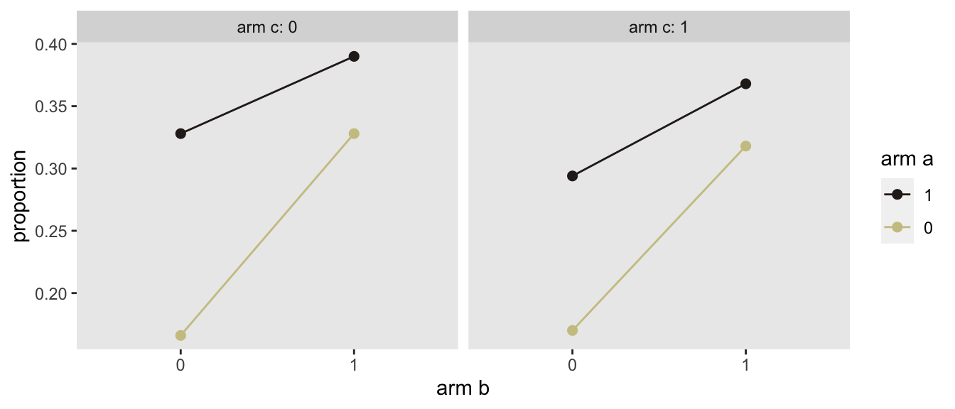
## 4000: 4000 0 1 0 1Here are the observed proportions by treatment arm. The fact that the two panels (\(c = 0\) and \(c = 1\)) are pretty similar are an indication that intervention \(c\) has no impact. And the fact that lines are not parallel in each panel are an indication that there is some interaction (in this case negative).

Model fitting
The Bayesian sampling is using four chains of length 2,500 (following 1,000 warm-up iterations for each), so the posterior distribution will be estimated with 10,000 total samples. The code for the Stan model can be found in the addendum.
dt_to_list <- function(dx) {

  N <- nrow(dx)
  x_abc <- model.matrix(~a*b*c, data = dx)
  y <- dx[, y]

  list(N = N, x_abc = x_abc, y = y)
}

mod <- cmdstan_model("code/model_ind.stan")

fit <- mod$sample(
  data = dt_to_list(dd),
  refresh = 0,
  chains = 4L,
  parallel_chains = 4L,
  iter_warmup = 1000,
  iter_sampling = 2500,
  adapt_delta = 0.98,
  max_treedepth = 20,
  show_messages = FALSE,
  seed = 29817
)
## Running MCMC with 4 parallel chains...
##
## Chain 1 finished in 113.5 seconds.
## Chain 3 finished in 124.9 seconds.
## Chain 4 finished in 129.5 seconds.
## Chain 2 finished in 130.2 seconds.
##
## All 4 chains finished successfully.
## Mean chain execution time: 124.5 seconds.
## Total execution time: 130.5 seconds.Presenting the results
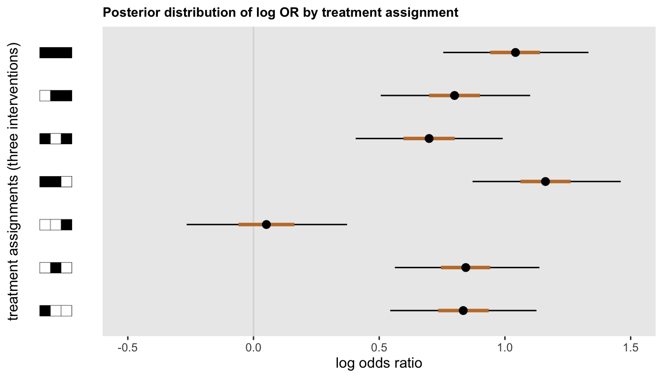
Here is the code for the first plot, which shows the distribution of effect sizes (on the log-odds scale) for each of the intervention arms. I’ve extracted the samples using the posterior package function as_draw_rvars that I recently described here.
posterior <- data.frame(as_draws_rvars(fit$draws(variables = "lOR")))

pcts <- c(.025, 0.25, .50, 0.75, .975)
sumstats <- data.table(t(quantile(posterior$lOR, pcts)))
setnames(sumstats, glue("p{pcts}"))
sumstats$var <- glue("lOR[{1:7}]")

p <- ggplot(data = sumstats, aes(y = var, yend = var)) +
  geom_vline(xintercept = 0, color = "grey85") +
  geom_segment(aes(x = p0.025, xend = p0.975)) +
  geom_segment(aes(x = p0.25, xend = p0.75),
    size = 1.25, color = palettes_d$wesanderson$Moonrise2[2]) +
  geom_point(aes(x = p0.5), size = 2.5) +
  theme(panel.grid = element_blank(),
        axis.text.y = element_blank(),
        axis.ticks.y = element_blank(),
        axis.title.y = element_text(margin = margin(t = 0, r = -12, b = 0, l = 0)),
        plot.title = element_text(size = 10, face = "bold")
  ) +
  ylab("treatment assignments (three interventions)") +
  xlab("log odds ratio") +
  xlim(-.5, 1.5) +
  ggtitle("Posterior distribution of log OR by treatment assignment")

pimage <- axis_canvas(p, axis = 'y') +
  draw_image("r_icons/r111.png", y = 6.5, scale = 0.35) +
  draw_image("r_icons/r011.png", y = 5.5, scale = 0.35) +
  draw_image("r_icons/r101.png", y = 4.5, scale = 0.35) +
  draw_image("r_icons/r110.png", y = 3.5, scale = 0.35) +
  draw_image("r_icons/r001.png", y = 2.5, scale = 0.35) +
  draw_image("r_icons/r010.png", y = 1.5, scale = 0.35) +
  draw_image("r_icons/r100.png", y = 0.5, scale = 0.35)
Looking at the figure, it is apparent that that \(a\) and \(b\) likely had an effect, while \(c\) probably did not. It also appears that the combination of \(a\) and \(b\) might be an improvement, both with and without \(c\):
ggdraw(insert_yaxis_grob(p, pimage, position = "left", width = grid::unit(.17, "null")))
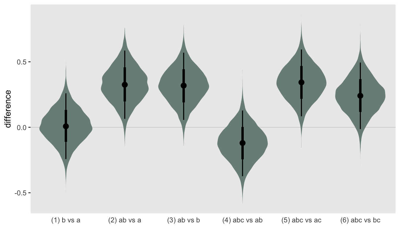
In the next and last plot, my goal is to compare the log-odds ratios of the different arms. I am showing the the posterior distributions for the differences between the estimated log-odds ratios. In this particular data set, \(a\) does not look any different from \(b\), but the combination of \(a\) and \(b\) does indeed look superior to either alone, regardless of whether \(c\) is involved:
data <- with(posterior, data.frame(
  x = c(
    "(1) b vs a",
    "(2) ab vs a",
    "(3) ab vs b",
    "(4) abc vs ab",
    "(5) abc vs ac",
    "(6) abc vs bc"
  ),
  diff = c(
    lOR[2] - lOR[1],
    lOR[4] - lOR[1],
    lOR[4] - lOR[2],
    lOR[7] - lOR[4],
    lOR[7] - lOR[5],
    lOR[7] - lOR[6]
  )
))

ggplot(data = data, aes(dist = diff, x = x)) +
  geom_hline(yintercept = 0, color = "grey80", size = .3) +
  stat_dist_eye(fill = palettes_d$wesanderson$Moonrise2[1], position="dodge") +
  theme(panel.grid = element_blank(),
        axis.title.x = element_blank(),
        axis.ticks.x = element_blank()) +
  ylab("difference")
Ultimately, how we present the data and draw our conclusions will depend on what we specify up front regarding the parameters and comparisons of interest. The great thing about a Bayesian model is that we have estimated everything in a single model, so there are no real concerns with multiple comparisons. However, reviewers still like to see results for analyses that were pre-specified. And if a decision is to be made based on those results, those decision rules should be pre-specified. But, my preference would be to show the findings and let readers decide if the results are compelling and/or determine if a more focused trial is needed.
In the next (and most likely, for now at least, final) post on this topic, I plan on describing how I approached sample size estimation for this proposed study.
Addendum
data {

  int<lower=0> N;                       // number patients
  matrix<lower=0, upper=1>[N, 8] x_abc;
  int<lower=0,upper=1> y[N];            // outcome for individual i

}

parameters {

  vector[8] z;

  real delta_m;
  real<lower = 0> sigma_m;

  real delta_x;
  real<lower=0> sigma_x;

}

transformed parameters {

  vector[8] tau;

  tau[1] = z[1];

  for (i in 2:4){
    tau[i] = sigma_m * z[i] + delta_m;
  }

  for (i in 5:7){
    tau[i] = sigma_x * z[i] + delta_x;
  }

  tau[8] = z[8];


}

model {

  sigma_m ~ student_t(3, 0, 2.5);
  sigma_x ~ student_t(3, 0, 2.5);

  delta_m ~ normal(0, 1);
  delta_x ~ normal(0, 1);

  z ~ std_normal();

  y ~ bernoulli_logit(x_abc * tau);

}

generated quantities {

  real lOR[7];

  lOR[1] = tau[2];                                            //  a=1, b=0, c=0
  lOR[2] = tau[3];                                            //  a=0, b=1, c=0
  lOR[3] = tau[4];                                            //  a=0, b=0, c=1
  lOR[4] = tau[2] + tau[3] + tau[5];                          //  a=1, b=1, c=0
  lOR[5] = tau[2] + tau[4] + tau[6];                          //  a=1, b=0, c=1
  lOR[6] = tau[3] + tau[4] + tau[7];                          //  a=0, b=1, c=1
  lOR[7] = tau[2]+tau[3]+tau[4]+tau[5]+tau[6]+tau[7]+tau[8];  //  a=1, b=1, c=1

}