Way back in 2018, long before the pandemic, I described a soon-to-be implemented simstudy function genMultiFac that facilitates the generation of multi-factorial study data. I followed up that post with a description of how we can use these types of efficient designs to answer multiple questions in the context of a single study.
Fast forward three years, and I am thinking about these designs again for a new grant application that proposes to study simultaneously three interventions aimed at reducing emergency department (ED) use for people living with dementia. The primary interest is to evaluate each intervention on its own terms, but also to assess whether any combinations seem to be particularly effective. While this will be a fairly large cluster randomized trial with about 80 EDs being randomized to one of the 8 possible combinations, I was concerned about our ability to estimate the interaction effects of multiple interventions with sufficient precision to draw useful conclusions, particularly if the combined effects of two or three interventions are less than additive. (That is, two interventions may be better than one, but not twice as good.)
I am thinking that a null hypothesis testing framework might not be so useful here, given the that the various estimates could be highly uncertain, not to mention the multiple statistical tests that we would need to conduct (and presumably adjust for). Rather, a Bayesian approach that pools estimates across interventions and provides posterior probability distributions may provide more insight into how the interventions interact could be a better way to go.
With this in mind, I went to the literature, and I found these papers by Kassler et al and Gelman. They both describe a way of thinking about interaction that emphasizes the estimates of variance across effect estimands. I went ahead and tested the idea with simulated data, which I’m showing here. Ultimately, I decided that this approach will not work so well for our study, and I came up with a pretty simple solution that I will share next time.
Identifying interaction through variance
The scenarios described by both papers involve studies that may be evaluating many possible interventions or exposures, each of which may have two or more levels. If we are dealing with a normally distributed (continuous) outcome measure, we can model that outcome as
where there are interventions, and intervention has levels. So, if intervention has 4 levels, is effectively the grand mean. are the mean contributions for the th intervention, and we constrain Again, for intervention , we would have with
The adjustments made for the two-way interactions are represented by the ’s through the ’s. If intervention 5 has levels then for the interaction between interventions 3 and 5 we have and
This pattern continues for higher orders of interaction (i.e. 3-way, 4-way, etc.).
In the Bayesian model, each set of ’s shares a common prior distribution with mean 0 and standard deviation :
where is a hyperparameter that will be estimated from the data. The same is true for the interaction terms for interventions and :
To assess whether there is interaction between the interventions (i.e. the effects are not merely additive), we are actually interested the variance parameters of the interaction . If, for example there is no interaction between different levels of interventions of 3 and 5, then should be close to , implying that . On the other hand, if there is some interaction effect, then implying that at least one
One advantage of the proposed Bayesian model is that we can use partial pooling to get more precise estimates of the variance terms. By this, I mean that we can use information from each to inform the others. So, in the case of 2-way interaction, the prior probability assumption would suggest that the the variance terms were drawn from a common distribution:
We can impose more structure (and hopefully precision) by doing the same for the main effects:
Of course, for each higher order interaction (above 2-way), we could impose the same structure:
And so on. Though at some point, we might want to assume that there is no higher order interaction and exclude it from the model; in most cases, we could stop at 2- or 3-way interaction and probably not sacrifice too much.
Example from simulation
When I set out to explore this model, I started relatively simple, using only two interventions with four levels each. In this case, the factorial study would have 16 total arms . (Since I am using only 2 interventions, I am changing the notation slightly, using interventions and rather than and .) Individual is randomized to one level in and one level , and and , and Using the same general model from above, here is the specific model for continuous :
Take note that we only have a single set of 2-way interactions since there are only two groups of interventions. Because of this, there is no need for a hyperparameter; however, there is a hyperparameter to pool across the main effects of and . Here are the prior distribution assumptions:
In order to ensure identifiability, we have the following constraints:
Required libraries
library(simstudy)
library(data.table)
library(cmdstanr)
library(caret)
library(posterior)
library(bayesplot)
library(ggdist)
library(glue)
Data generation
The parameters are set so that there is greater variation in treatment compared to treatment . In both cases, the sum of the parameters is set to .
t_0 <- 0
t_a <- c(-8, -1, 3, 6)
t_b <- c(-3, -1, 0, 4)
The interaction is set in this case so that there is an added effect when both and . Again, the parameters are set so that the sum-to-zero constraint is maintained.
x <- c(4, 3)
nox <- - sum(x) / (16 - length(x))

t_ab <- matrix(c(nox, nox, nox, nox,
                 nox,   4, nox, nox,
                 nox,   3, nox, nox,
                 nox, nox, nox, nox), nrow = 4, byrow = TRUE)

t_ab
## [,1] [,2] [,3] [,4]
## [1,] -0.5 -0.5 -0.5 -0.5
## [2,] -0.5 4.0 -0.5 -0.5
## [3,] -0.5 3.0 -0.5 -0.5
## [4,] -0.5 -0.5 -0.5 -0.5sum(t_ab)## [1] 0The data definitions for the arm assignments and the outcome are established using the simstudy package:
d1 <- defDataAdd(varname = "y", formula = "mu", variance = 16, dist = "normal")Now we are ready to generate the data:
set.seed(110)

dd <- genMultiFac(nFactors = 2, levels = 4, each = 30, colNames = c("a", "b"))
dd[, mu := t_0 + t_a[a] + t_b[b] + t_ab[a, b], keyby = id]
dd <- addColumns(d1, dd)
Plot of by arm
The plot shows the the average outcomes by arm. The interaction when and is apparent in the two locations where the smooth pattern of increases is interrupted.
## Warning: Using `size` aesthetic for lines was deprecated in ggplot2 3.4.0.
## ℹ Please use `linewidth` instead.
## This warning is displayed once every 8 hours.
## Call `lifecycle::last_lifecycle_warnings()` to see where this warning was
## generated.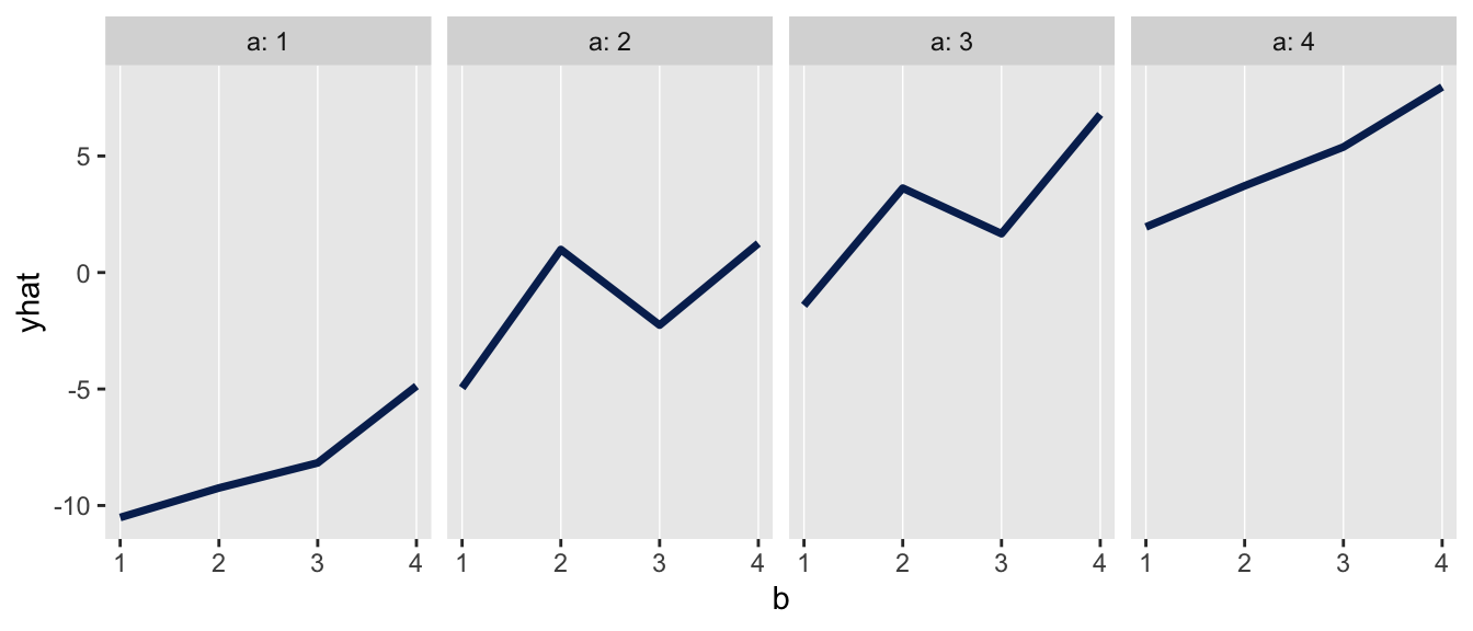
Sampling from the posterior
The function shown next simply generates the data needed by Stan. (The Stan implementation is shown below in the addendum.) Take note that we convert the design matrix of 0’s and 1’s to a single vector with values ranging from 1 to 16.
dt_to_list <- function(dx) {

  dx[, a_f := factor(a)]
  dx[, b_f := factor(b)]

  dv <- dummyVars(~ b_f:a_f , data = dx, n = c(4, 4))
  dp <- predict(dv, dx )

  N <- nrow(dx)                               ## number of observations
  I <- 2
  X2 <- 1

  main <- as.matrix(dx[,.(a,b)])

  ab <- as.vector(dp %*% c(1:16))
  x <- as.matrix(ab, nrow = N, ncol = X2)

  y <- dx[, y]

  list(N=N, I=I, X2=X2, main=main, x=x, y=y)

}
I am using cmdstanr to interact with Stan:
mod <- cmdstan_model("code/model_2_factors.stan", force_recompile = TRUE)

fit <- mod$sample(
  data = dt_to_list(dd),
  refresh = 0,
  chains = 4L,
  parallel_chains = 4L,
  iter_warmup = 500,
  iter_sampling = 2500,
  adapt_delta = 0.99,
  step_size = .05,
  max_treedepth = 20,
  seed = 1721
)
Diagnostic checks
Here is just one set of trace plots for that indicate the sampling went quite well - the variables not shown were equally well-behaved.
posterior <- as_draws_array(fit$draws())
mcmc_trace(posterior, pars = glue("t[{1},{1:4}]"))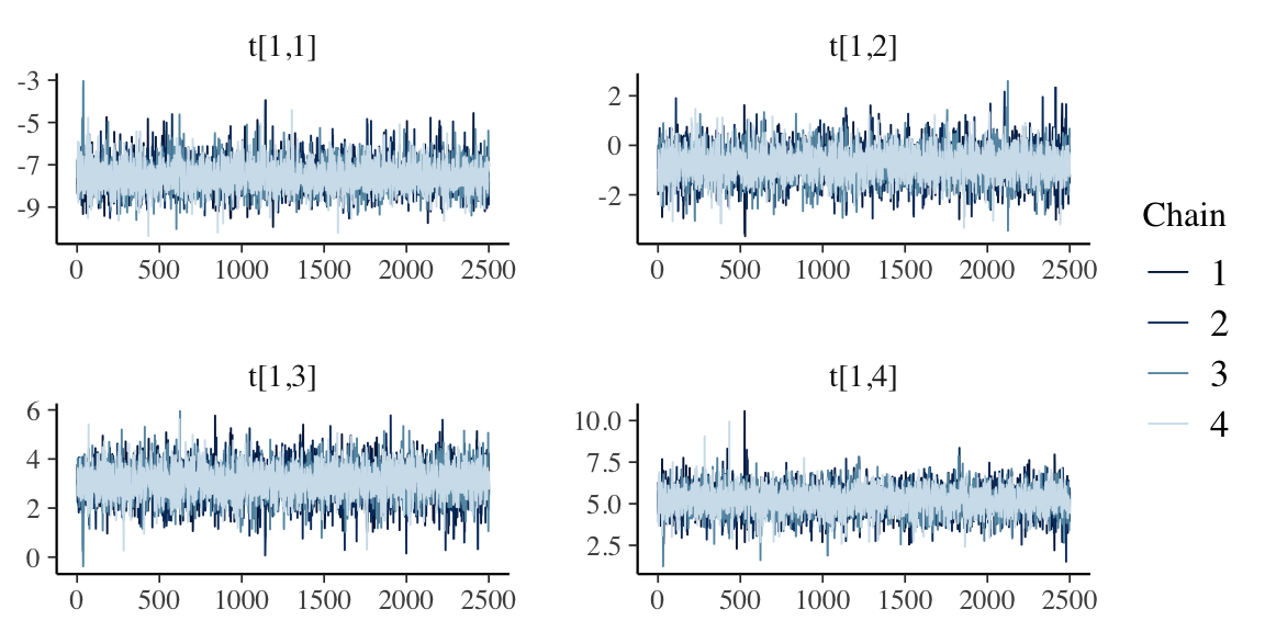
Variance estimates
Since we are focused on the possibility of 2-way interaction, the primary parameter of interest is the variation of the interaction effects. (In the Stan model specification this variance parameter is sigma_x, as in interaction.) The plot shows the 95% credible intervals for each of the main effect variance parameters as well as the interaction variance parameter.
The fact that the two main effect variance parameters ( and ) are greater than zero supports the data generation process which assumed different outcomes for different levels of interventions and , respectively.
And the credible interval for (sigma_x), likewise is shifted away from zero, suggesting there might be some interaction between and at certain levels of each.
mcmc_intervals(posterior, pars = c(glue("sigma_m[{1:2}]"), "sigma_x[1]"))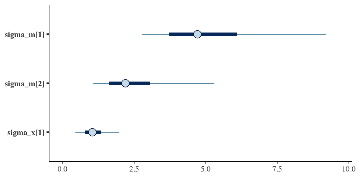
We can hone in a bit more on the specific estimates of the ’s to see where those interactions might be occurring. It appears that t_x[1,6] (representing ) is an important interaction term - which is consistent with the data generation process. However, , represented by t_x[1,10] is not obviously important. Perhaps we need more data.
mcmc_intervals(posterior, pars = glue("t_x[1,{1:16}]"))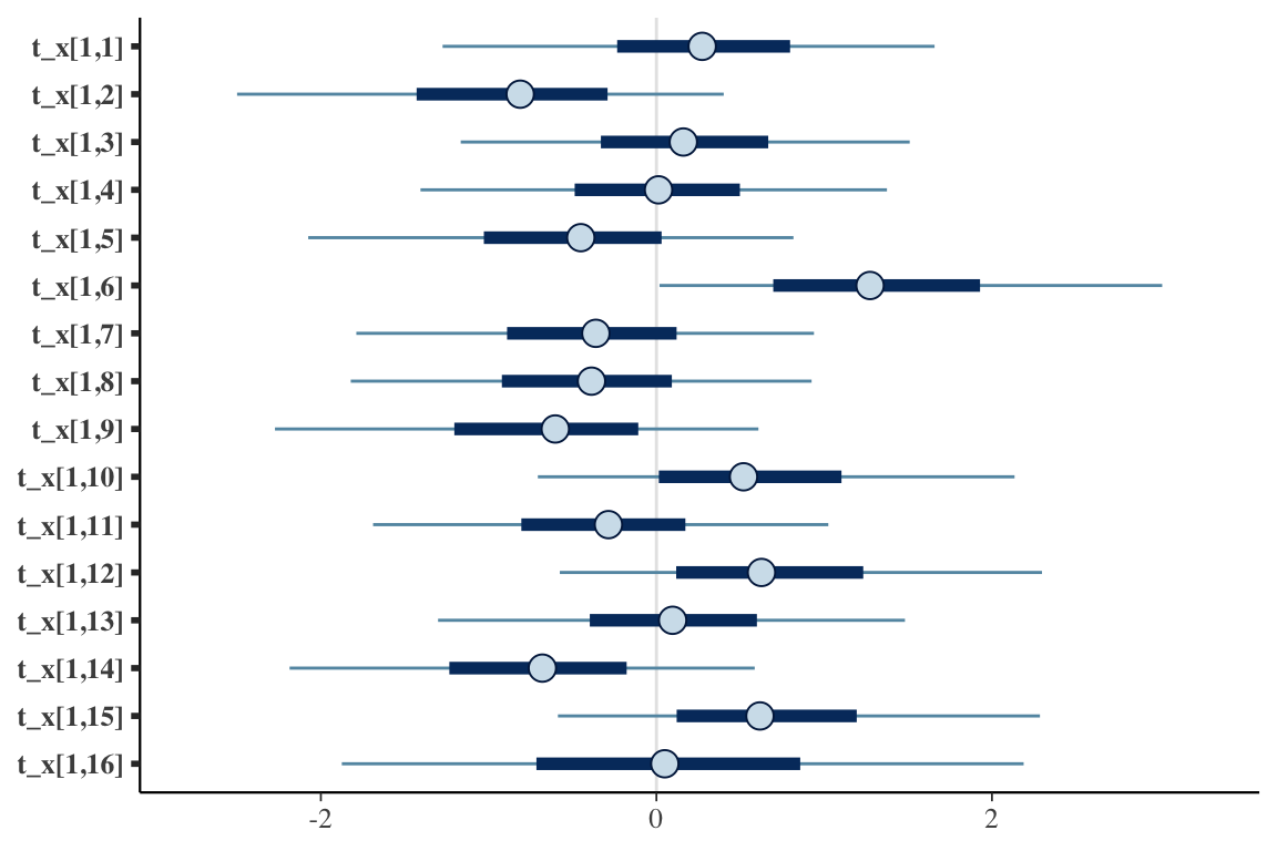
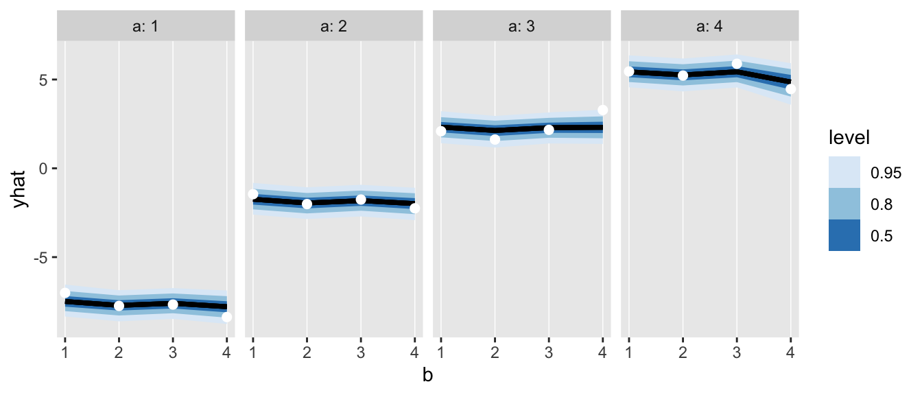
Below is a visual representation of how well the model fits the data by showing the interval of predicted cell counts for each pair. The observed means (shown as white dots) sit on top of the predictions (shown by the colored lines), suggesting the model is appropriate.
r <- as_draws_rvars(fit$draws(variables = c("t_0","t", "t_x")))

dnew <- data.frame(
  genMultiFac(nFactors = 2, levels = 4, each = 1, colNames = c("b", "a")))

dnew$yhat <- with(r,
  rep(t_0, 16) + rep(t[1, ], each = 4) + rep(t[2, ], times = 4) + t(t_x))

ggplot(data = dnew, aes(x=b, dist = yhat)) +
  geom_vline(aes(xintercept = b), color = "white", size = .25) +
  stat_dist_lineribbon() +
  geom_point(data = dsum, aes(y = yhat), color = "white", size = 2) +
  facet_grid(.~a, labeller = labeller(a = label_both)) +
  theme(panel.grid.minor = element_blank(),
        panel.grid.major = element_blank())  +
  scale_fill_brewer()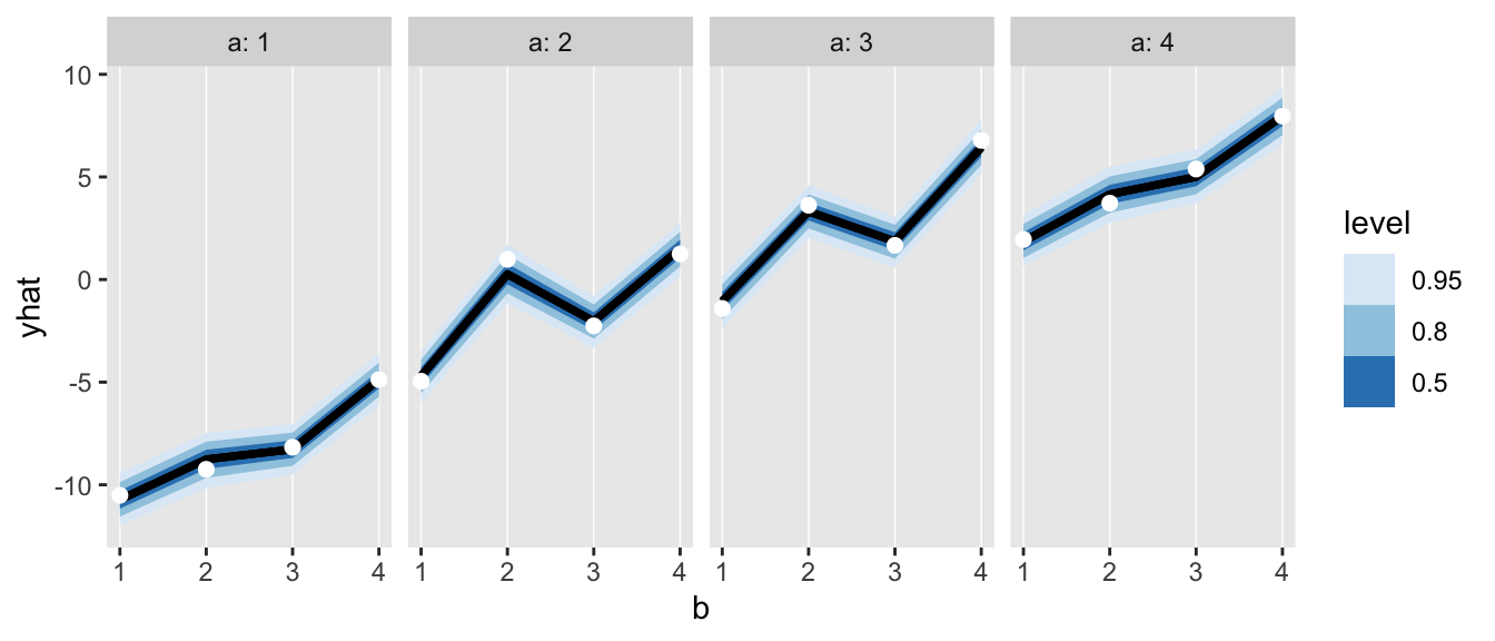
Only one treatment effect and no interaction
Perhaps the rationale for focusing on the variance can be best appreciated by looking at a contrasting scenario where there is only a single main effect (for intervention ) and no interaction. Here we would expect the estimates for the intervention main effects variance as well as the variance of the interaction terms to be close to zero.
t_0 <- 0
t_a <- c(-8, -1, 3, 6)
t_b <- c(0, 0, 0, 0)
t_ab <- matrix(0, nrow = 4, ncol = 4)
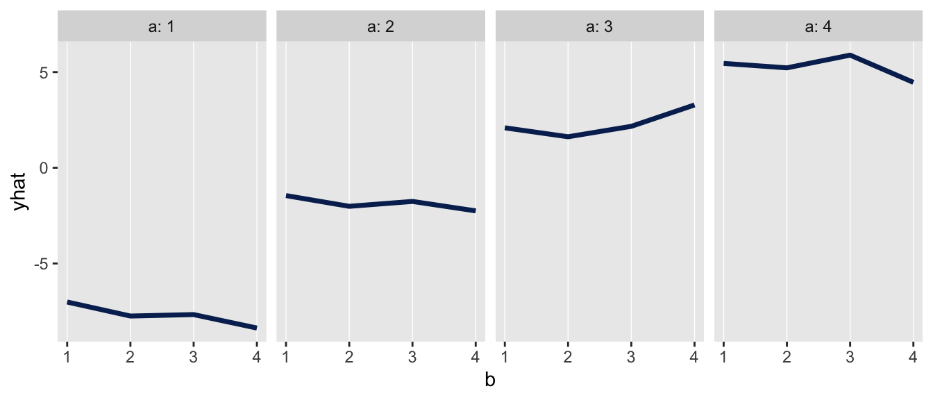
The plot of the observed means is consistent with the data generation process:
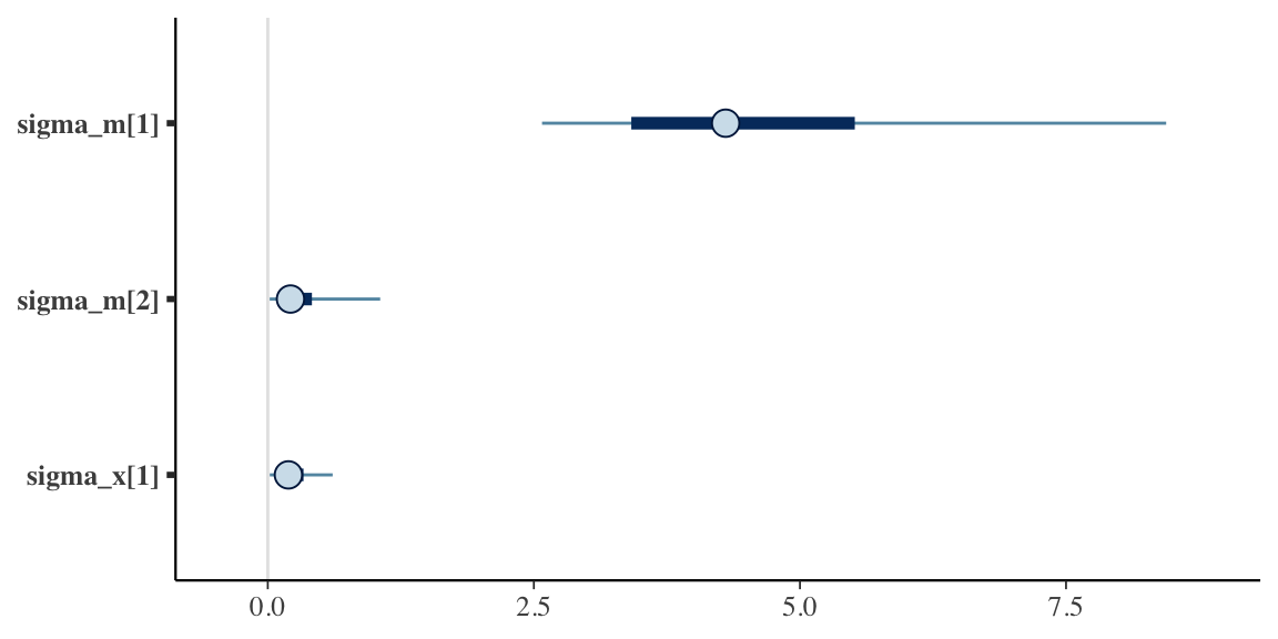
And yes, the posterior distribution for (sigma_x) is now very close to zero …
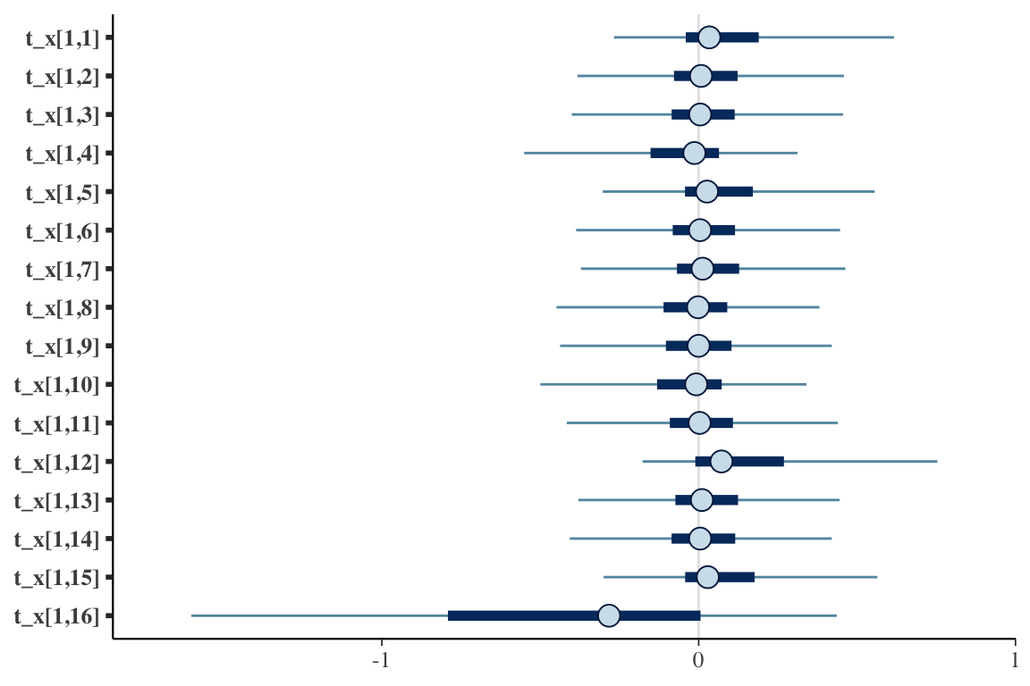
and the effect parameters are all centered around zero:
Once again, the predicted values are quite close to the observed means - indicating the model is a good fit:
Next steps
In the motivating application, there are actually three interventions, but each one has only two levels (yes or no). In this case, the level mean and across-level variance parameters were poorly estimated, probably because there are so few levels. This forced me to take a more traditional approach, where I estimate the means of each randomization arm. I’ll share that next time.
References:
Gelman, Andrew. “Analysis of variance—why it is more important than ever.” The annals of statistics 33, no. 1 (2005): 1-53.
Kassler, Daniel, Ira Nichols-Barrer, and Mariel Finucane. “Beyond “treatment versus control”: How Bayesian analysis makes factorial experiments feasible in education research.” Evaluation review 44, no. 4 (2020): 238-261.
Addendum
The model is implemented in Stan using a non-centered parameterization, so that the parameters are a function of a set of parameters, which are standard normal parameters. This does not dramatically change the estimates, but eliminates divergent chains, improving sampling behavior.
data {

  int<lower=1> N;        // number of observations
  int<lower=1> I;        // number of interventions
  int<lower=1> X2;       // number of 2-way interactions
  array[N, I] int main;  // interventions
  array [N, X2] int x;   // interactions - provide levels for each intervention?

  vector[N] y;           // outcome

}

parameters {

  real t_0;

  array[I] vector[3] z_raw;
  array[X2] vector[15] z_x_raw;

  real<lower=0> sigma;
  array[I] real<lower=0> sigma_m;
  array[X2] real<lower=0> sigma_x;

  real<lower=0> sigma_main;

}

transformed parameters {

  // constrain parameters to sum to 0

  array[I] vector[4] z;
  array[X2] vector[16] z_x;

  array[I] vector[4] t;
  array[X2] vector[16] t_x;

  vector[N] yhat;

  for (i in 1:I) {
    z[i] = append_row(z_raw[i], -sum(z_raw[i]));
  }

  for (i in 1:X2) {
    z_x[i] = append_row(z_x_raw[i], -sum(z_x_raw[i]));
  }

  for (i in 1:I)
     for (j in 1:4)
        t[i, j] = sigma_m[i] * z[i, j];

  for (i in 1:X2)
     for (j in 1:16)
        t_x[i, j] = sigma_x[i] * z_x[i, j];

  // yhat

  for (n in 1:N) {
    real ytemp;
    ytemp = t_0;
    for (i in 1:I) ytemp = ytemp + t[i, main[n, i]]; // 2 sets of main effects
    for (i in 1:X2) ytemp = ytemp + t_x[i, x[n, i]]; // 1 set of interaction effects
    yhat[n] = ytemp;
  }
}

model {

  sigma ~ normal(0, 5);
  sigma_m ~ normal(0, sigma_main);
  sigma_x ~ normal(0, 5);

  sigma_main ~ normal(0, 5);

  t_0 ~ normal(0, 5);

  for (i in 1:I) z_raw[i] ~ std_normal();
  for (i in 1:X2) z_x_raw[i] ~ std_normal();

  y ~ normal(yhat, sigma);

}