Say we’ve collected data and estimated parameters of a model that give structure to the data. An important question to ask is whether the model is a reasonable approximation of the true underlying data generating process. If we did a good job, we should be able to turn around and generate data from the model itself that looks similar to the data we started with. And if we didn’t do such a great job, the newly generated data will diverge from the original.
If we used a Bayesian approach to estimation, all the information we have about the parameters from our estimated model is contained in the data that have been sampled by the MCMC process. For example, if we are estimating a simple normal regression model with an intercept parameter , a slope parameter , and a standard deviation parameter , and we collected 10,000 samples from a posterior distribution, then we will have a multivariate table of possible values of , and . To answer our question regarding model adequacy, we only need to extract the information contained in all that data.
I’ve been casting about for ways to do this extraction efficiently in R, so I posted an inquiry on the Stan Forums to get advice. I got a suggestion to look into the random variable dataytpe (rvar) recently implemented in the package `posterior. Not at all familiar with this, I started off by reading through the vignette, and then at this Kerman & Gelman paper.
To get a get a better handle on the ideas and tools, I decided to simulate some data, fit some models, and investigate what posterior probability checks might like look using rvars. I’m sharing some of the code with you here to give a bit of the flavor of what can be done. A little advanced warning: I am providing more output of the data than usual, because I think it is easier to grasp what is going on if you can see the data in the various stages of transformation.
Before I get started, here is the requisite list of the packages needed to run the code:
library(simstudy)
library(data.table)
library(cmdstanr)
library(posterior)
library(bayesplot)
library(ggplot2)
library(abind)
Simple linear model
I am first generating data from a simple linear regression model where the outcome is a function of , and , , and :
Data generation
To get things going, I define the relationship between and and generate the data using simstudy, and then take a look at the data:
b_quad <- 0

ddef <- defData(varname = "x", formula = "0;10", dist = "uniform")
ddef <- defData(ddef, "y", "2 + 6*x + ..b_quad*(x^2)", 4)

set.seed(2762)
dd <- genData(100, ddef)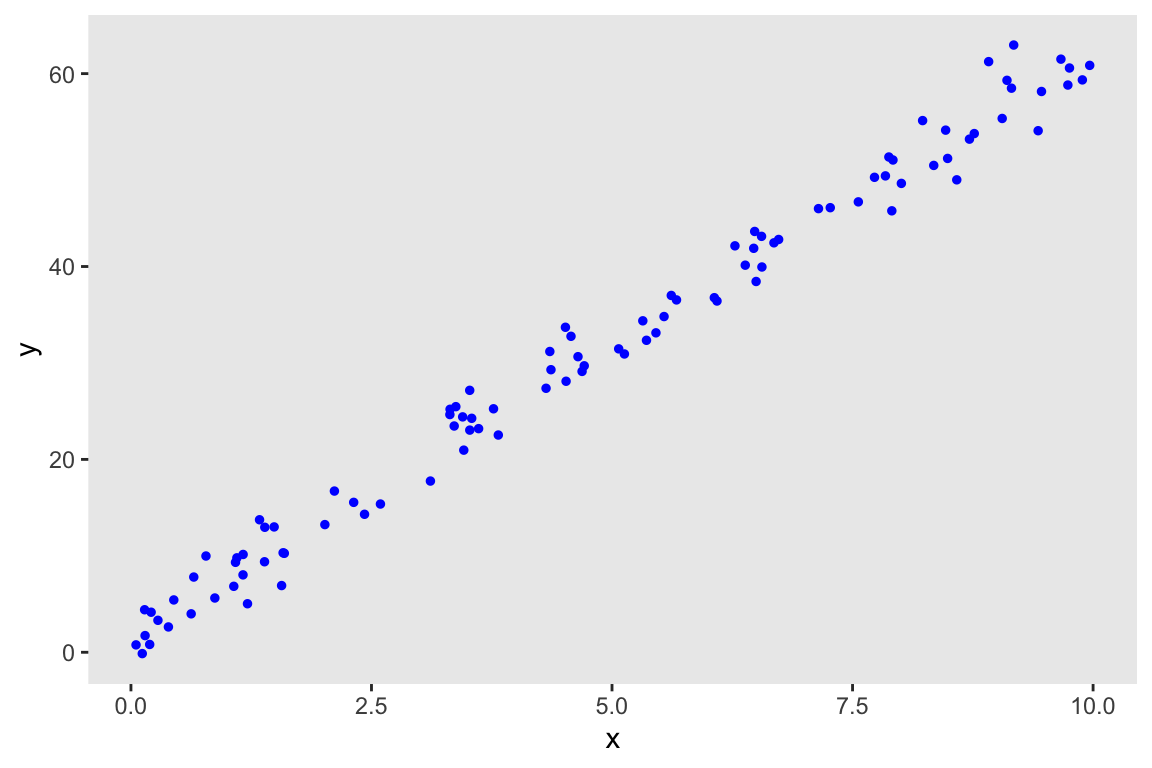
Model fitting
I am using cmdstan and cmdstanr to estimate the model. Here is the Stan code:
data {
  int<lower=0> N;
  vector[N] x;
  vector[N] y;
}

parameters {
  real alpha;
  real beta;
  real<lower=0> sigma;
}

model {
  y ~ normal(alpha + beta*x, sigma);
}
Next, I compile the Stan code, and sample from the posterior. The sampling will be done in four parallel chains of 2,500 (after the warm-up of 500 samples), which will give me a total sample of 10,000 for each parameter. All of the samples are stored in the cmdstan object fit.
mod <- cmdstan_model("code/linear_regression.stan")fit <- mod$sample(
data = list(N = nrow(dd), x = dd$x, y = dd$y),
seed = 93736,
refresh = 0,
chains = 4L,
parallel_chains = 4L,
iter_warmup = 500,
iter_sampling = 2500
)## Running MCMC with 4 parallel chains...
##
## Chain 1 finished in 0.1 seconds.
## Chain 2 finished in 0.1 seconds.
## Chain 3 finished in 0.1 seconds.
## Chain 4 finished in 0.1 seconds.
##
## All 4 chains finished successfully.
## Mean chain execution time: 0.1 seconds.
## Total execution time: 0.2 seconds.Extracting results
Typically, I would extract the data using the draws method of the cmdstanr object. By default, the draws method returns an array, which is essentially (though not exactly) a multi-dimensional matrix. In this case there are multiple matrices, one for each parameter. The display of each parameter shows the first five rows of the four chains.
(post_array <- fit$draws())## # A draws_array: 2500 iterations, 4 chains, and 4 variables
## , , variable = lp__
##
## chain
## iteration 1 2 3 4
## 1 -128 -129 -127 -128
## 2 -128 -128 -127 -128
## 3 -128 -129 -130 -128
## 4 -128 -128 -127 -129
## 5 -128 -127 -127 -128
##
## , , variable = alpha
##
## chain
## iteration 1 2 3 4
## 1 2.1 1.5 2.0 2.4
## 2 1.6 1.7 1.8 2.3
## 3 1.7 2.2 1.7 2.4
## 4 1.5 2.5 1.7 1.3
## 5 2.0 2.1 1.6 2.2
##
## , , variable = beta
##
## chain
## iteration 1 2 3 4
## 1 6.1 6.2 6.0 6.0
## 2 6.0 6.1 6.1 6.0
## 3 6.1 5.9 6.1 5.9
## 4 6.1 6.0 6.1 6.1
## 5 6.0 6.0 6.1 6.0
##
## , , variable = sigma
##
## chain
## iteration 1 2 3 4
## 1 2.0 2.4 2.0 2.1
## 2 2.0 2.2 2.0 2.4
## 3 2.3 2.3 1.8 2.3
## 4 2.2 2.2 2.1 2.1
## 5 2.3 2.3 2.3 2.5
##
## # ... with 2495 more iterationsThe package bayesplot uses this array to generate a range of different plots, including the important diagnostic trace plot:
mcmc_trace(post_array, pars = c("alpha", "beta", "sigma"), facet_args = list(nrow = 3))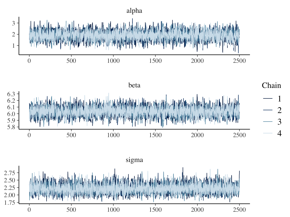
Random variable datatype
Instead of extracting the array data, it is possible to convert the array into a random variable datatype, or rvar. It is probably easiest to explain what this is by looking more closely at it.
(post_rvars <- as_draws_rvars(fit$draws()))## # A draws_rvars: 2500 iterations, 4 chains, and 4 variables
## $lp__: rvar<2500,4>[1] mean ± sd:
## [1] -128 ± 1.2
##
## $alpha: rvar<2500,4>[1] mean ± sd:
## [1] 1.9 ± 0.41
##
## $beta: rvar<2500,4>[1] mean ± sd:
## [1] 6 ± 0.072
##
## $sigma: rvar<2500,4>[1] mean ± sd:
## [1] 2.2 ± 0.16You can see that the post_rvars object is essentially a list of 4 items: lp (log probability), alpha, beta, and sigma. But what exactly are those items, “1.9 ± 0.41” for alpha, “6 ± 0.072” for beta, and “2.2 ± 0.16” for sigma? Well, the rvar is really a shorthand way of representing the detailed data that is in the underlying array, and the text displayed is merely the mean and standard deviation of the underlying data (). We can peek under the hood a bit by using the function draws_of, and confirm the mean and standard deviation of the samples:
beta_samples <- draws_of(post_rvars$beta)
data.table(beta_samples)
## V1
## 1: 6.07
## 2: 6.04
## 3: 6.13
## 4: 6.14
## 5: 5.98
## ---
## 9996: 6.00
## 9997: 6.07
## 9998: 6.03
## 9999: 6.13
## 10000: 6.14c(mean(beta_samples), sd(beta_samples))## [1] 6.0350 0.0715Why all the fuss?
The whole point of the rvar datatype is that it makes it much easier to do things like estimate the distributions of the functions of the parameters and to generate predicted values of new observations, both things we need for posterior probability checking. Of course, there are other ways to do all of this (as is always the case in R), but thisrvars` seem to eliminate a lot of the manipulation that might be necessary if we chose to work directly with the data arrays.
In this next step, I am generating the distribution of means for each of the 100 individuals in the data set:
I want to do this, because ultimately, I want to generate predicted values for each individual, which come from . And I am not going to generate just a single predicted value for each individual, but rather 10,000 predicted values for each individual. So, now we will have the distribution of predicted values for each individual, which is quite powerful. And importantly, the distributions of these predicted values will incorporate the uncertainty of each and . With the rvar datatype, all of this can be accomplished with just a few commands - no manipulation necessary.
All rvar equations need to be specified using by rvar objects. We need the product of and to get , but is observed data, not a random variable. No problem - we can covert the vector into a special kind of constant rvar that does not have a standard deviation. Once this is done, we can generate the ’s
x_rvar <- as_rvar(dd$x)
x_rvar
## rvar<1>[100] mean ± sd:
## [1] 6.554 ± NA 0.281 ± NA 2.115 ± NA 9.889 ± NA 8.715 ± NA
## [6] 3.448 ± NA 5.358 ± NA 1.069 ± NA 7.908 ± NA 0.445 ± NA
## [11] 4.574 ± NA 1.581 ± NA 8.915 ± NA 6.063 ± NA 6.278 ± NA
## [16] 7.146 ± NA 8.344 ± NA 6.385 ± NA 9.429 ± NA 1.391 ± NA
## [21] 3.542 ± NA 6.473 ± NA 4.689 ± NA 2.016 ± NA 3.818 ± NA
## [26] 1.566 ± NA 3.315 ± NA 0.118 ± NA 3.317 ± NA 4.523 ± NA
## [31] 4.711 ± NA 1.488 ± NA 8.488 ± NA 3.614 ± NA 3.521 ± NA
## [36] 0.653 ± NA 3.522 ± NA 5.541 ± NA 3.377 ± NA 0.142 ± NA
## [41] 0.626 ± NA 1.211 ± NA 5.616 ± NA 0.210 ± NA 5.320 ± NA
## [46] 3.459 ± NA 2.315 ± NA 6.498 ± NA 9.055 ± NA 6.483 ± NA
## [51] 1.087 ± NA 2.593 ± NA 8.007 ± NA 1.388 ± NA 7.268 ± NA
## [56] 1.101 ± NA 6.091 ± NA 7.920 ± NA 4.646 ± NA 7.842 ± NA
## [61] 3.113 ± NA 7.560 ± NA 6.683 ± NA 5.670 ± NA 8.468 ± NA
## [66] 9.152 ± NA 0.390 ± NA 4.365 ± NA 8.228 ± NA 6.732 ± NA
## [71] 4.516 ± NA 1.166 ± NA 6.558 ± NA 5.129 ± NA 9.666 ± NA
## [76] 4.314 ± NA 5.069 ± NA 0.872 ± NA 7.728 ± NA 0.780 ± NA
## [81] 0.053 ± NA 1.594 ± NA 5.457 ± NA 9.755 ± NA 0.147 ± NA
## [86] 8.765 ± NA 1.165 ± NA 9.738 ± NA 0.195 ± NA 9.965 ± NA
## [91] 9.175 ± NA 8.583 ± NA 9.464 ± NA 3.360 ± NA 3.768 ± NA
## [96] 9.105 ± NA 1.337 ± NA 7.878 ± NA 4.354 ± NA 2.428 ± NAmu <- post_rvars$alpha + post_rvars$beta * x_rvar
mu## rvar<2500,4>[100] mean ± sd:
## [1] 41.5 ± 0.25 3.6 ± 0.39 14.7 ± 0.29 61.6 ± 0.43 54.5 ± 0.36
## [6] 22.7 ± 0.24 34.2 ± 0.22 8.4 ± 0.34 49.6 ± 0.31 4.6 ± 0.38
## [11] 29.5 ± 0.22 11.5 ± 0.32 55.7 ± 0.37 38.5 ± 0.24 39.8 ± 0.24
## [16] 45.0 ± 0.28 52.3 ± 0.34 40.4 ± 0.25 58.8 ± 0.40 10.3 ± 0.33
## [21] 23.3 ± 0.24 41.0 ± 0.25 30.2 ± 0.22 14.1 ± 0.30 25.0 ± 0.23
## [26] 11.4 ± 0.32 21.9 ± 0.24 2.6 ± 0.40 21.9 ± 0.24 29.2 ± 0.22
## [31] 30.3 ± 0.22 10.9 ± 0.32 53.1 ± 0.34 23.7 ± 0.23 23.2 ± 0.24
## [36] 5.9 ± 0.37 23.2 ± 0.24 35.4 ± 0.23 22.3 ± 0.24 2.8 ± 0.40
## [41] 5.7 ± 0.37 9.2 ± 0.34 35.8 ± 0.23 3.2 ± 0.39 34.0 ± 0.22
## [46] 22.8 ± 0.24 15.9 ± 0.28 41.1 ± 0.25 56.6 ± 0.38 41.0 ± 0.25
## [51] 8.5 ± 0.34 17.6 ± 0.27 50.2 ± 0.32 10.3 ± 0.33 45.8 ± 0.28
## [56] 8.6 ± 0.34 38.7 ± 0.24 49.7 ± 0.31 30.0 ± 0.22 49.2 ± 0.31
## [61] 20.7 ± 0.25 47.5 ± 0.30 42.2 ± 0.26 36.1 ± 0.23 53.0 ± 0.34
## [66] 57.1 ± 0.38 4.3 ± 0.38 28.3 ± 0.22 51.6 ± 0.33 42.5 ± 0.26
## [71] 29.2 ± 0.22 8.9 ± 0.34 41.5 ± 0.25 32.9 ± 0.22 60.2 ± 0.41
## [76] 28.0 ± 0.22 32.5 ± 0.22 7.2 ± 0.36 48.6 ± 0.30 6.6 ± 0.36
## [81] 2.2 ± 0.40 11.5 ± 0.32 34.8 ± 0.22 60.8 ± 0.42 2.8 ± 0.40
## [86] 54.8 ± 0.36 8.9 ± 0.34 60.7 ± 0.42 3.1 ± 0.40 62.1 ± 0.43
## [91] 57.3 ± 0.38 53.7 ± 0.35 59.0 ± 0.40 22.2 ± 0.24 24.7 ± 0.23
## [96] 56.9 ± 0.38 10.0 ± 0.33 49.5 ± 0.31 28.2 ± 0.22 16.6 ± 0.28We can see that mu is an rvar vector of 100 objects, one for each individual . But, as we saw before, each of those objects is actually 10,000 data points - the distribution of for each individual. Again, let’s peek under the hood: here is the the distribution of for individual :
data.table(draws_of(mu[6]))## V1
## 1: 23.0
## 2: 22.4
## 3: 22.8
## 4: 22.7
## 5: 22.6
## ---
## 9996: 22.9
## 9997: 22.4
## 9998: 22.1
## 9999: 22.8
## 10000: 22.8Now we are ready to generate the distribution of predicted values for each individual - again using a single command rvar_rng, specifying that we want to generate data for each individual using the distribution of the rvar mu and the the rvar sigma. We get 10,000 predicted values (our estimated distribution) for each of the 100 individuals:
pred <- rvar_rng(rnorm, nrow(dd), mu, post_rvars$sigma)
str(pred)
## rvar<2500,4>[100] 41.4 ± 2.2 3.6 ± 2.2 14.7 ± 2.2 61.6 ± 2.3 ...Here, I randomly sample from the sample of 10,000 predicted values and plot this one instance of predicted values (in orange) along with the original data (in blue):
newdd <- data.table(x = dd$x, y = draws_of(pred)[sample(10000, 1),])
head(newdd)
## x y
## 1: 6.554 44.17
## 2: 0.281 2.57
## 3: 2.115 16.13
## 4: 9.889 60.41
## 5: 8.715 56.27
## 6: 3.448 24.04ggplot(data = dd, aes(x = x, y = y)) +
geom_point(color = "blue", size = 1) +
geom_point(color = "orange", size = 1, data = newdd) +
theme(panel.grid = element_blank())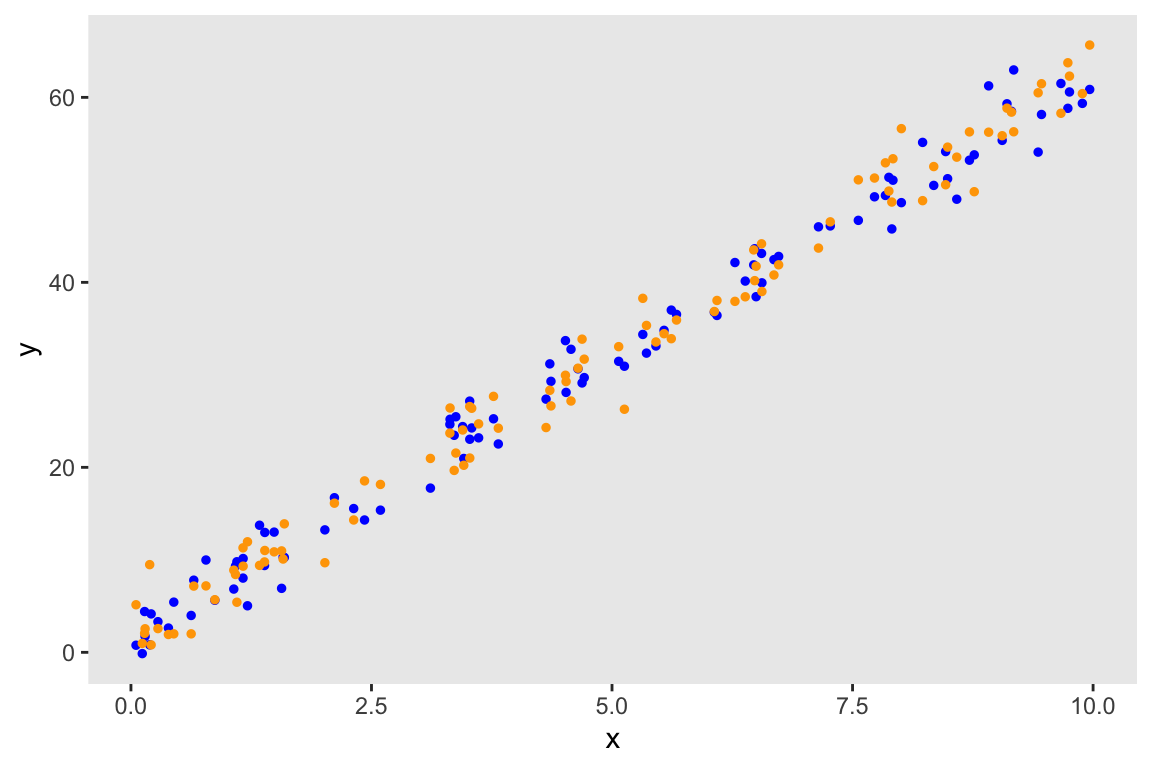
But we can actually visualize the distribution of predicted values for each individual and plot those distributions in relation to the actual data. If we want to look at the 80% interval for each individual (we could look at the 95% interval just as easily), we can estimate the interval bounds simply by applying the quantile function to the rvar pred:
interval80 <- t(quantile(pred, c(0.10, 0.90)))
head(interval80)
## [,1] [,2]
## [1,] 38.58 44.21
## [2,] 0.79 6.44
## [3,] 11.79 17.52
## [4,] 58.75 64.45
## [5,] 51.55 57.44
## [6,] 19.89 25.55If the model is a good fit, we would expect the actual data to be scattered across those distributions without any obvious pattern, as is the case here. Not so surprising given the simulated data generation process:
df.80 <- data.table(x = dd$x, y=dd$y, interval80)
df.80[, extreme := !(y >= V1 & y <= V2)]

ggplot(data = df.80, aes(x = x, y = y)) +
  geom_segment(aes(y = V1, yend = V2, x = x, xend = x), color = "grey30", size = .1) +
  geom_point(aes(color = extreme), size = 1) +
  theme(panel.grid = element_blank(),
        legend.position = "none") +
  scale_color_manual(values = c("black", "red"))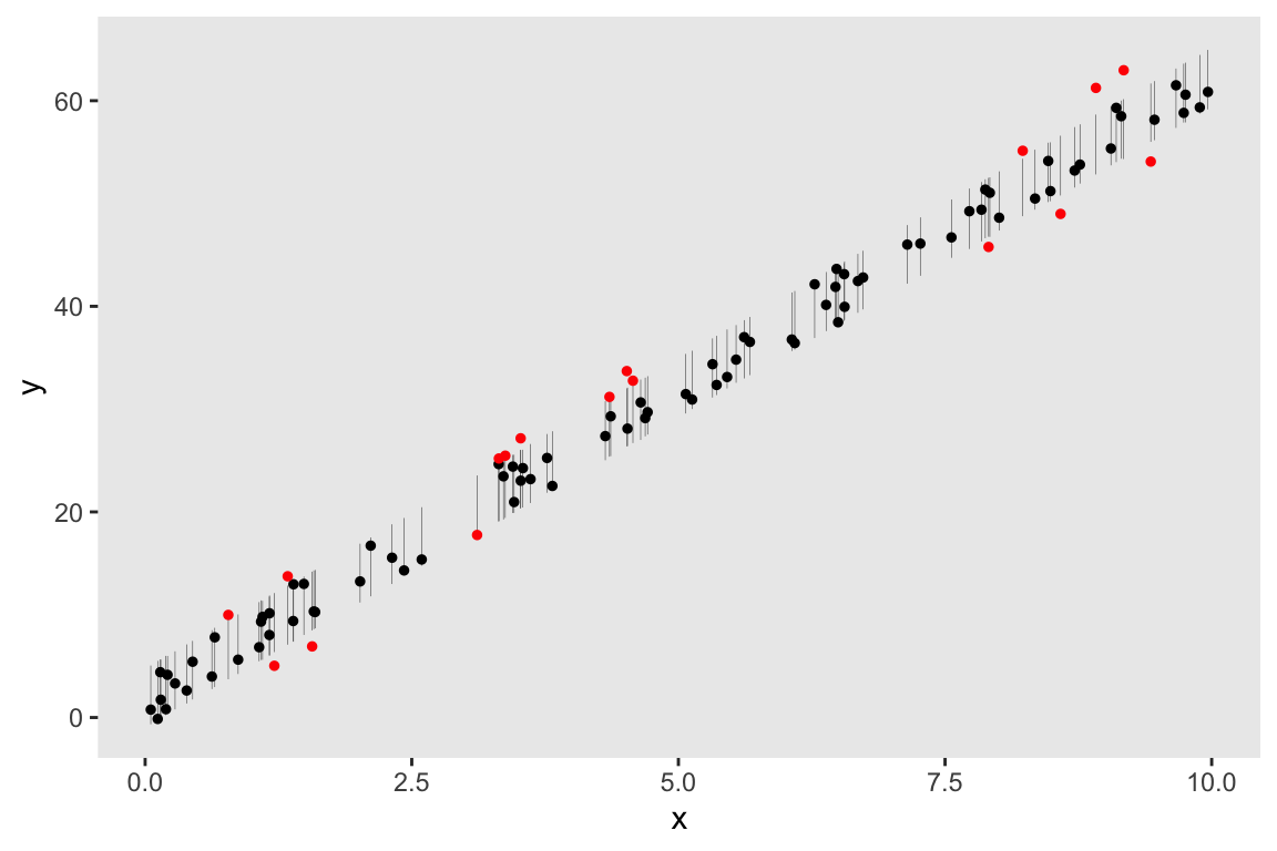
Bayesian p-value
I find the visual presentation pretty compelling, but if we want to quantify the model fit, one option is to estimate a Bayesian p-value, described in this Gelman paper as
averaged over the parameters (and is a function of the observed data ). is the replicated or predicted data from the model (what we have saved in the variable pred). is any function of the data that is reasonable in this context. The idea is that the p-value will not be extremely high or low (eg., not less than 0.05 or not greater than 0.95) if the model is a good approximation of the actual data generating process. Since my main goal here is to illustrate the usefulness of the rvar datatype, and not necessarily to come up with the ideal test statistic , I’ve created a pretty crude idea for in the the context of linear regression.
The first step is to split the data defined by different values of predictors into different bins (in this case I’ll use five) and calculate the proportion of observed ’s that fall below the predicted mean :
We also do the same to estimate for each bin, using the replicated/predicted values of . We expect the variability (i.e. ): by definition, predictions are randomly scattered around the means in each bin, with half above and half below. If the model is a good fit of the observed data, we would expect the ’s of based on observed data to all also be close to 0,5. However, if the model is a poor fit, there will likely be variability in proportions based on observed ’s across bins, so that the should be quite close to 0.
[As I write this, I’m noticing that this binned test statistic might bear some of the same motivations that underlie the Goldfeld-Quandt test for heteroscedasticity. OK, not quite, but perhaps it is very, very tangentially related? In any case, the more famous test was developed in part by my father; today would have been his 81st birthday, so I am very happy to make that (very subtle) connection.]
Estimating the p-value from the data
One cool feature of rvars is that they can be included in data.frames (though not in data.tables). This allows us to do some cool summarization without a lot of manipulation.
df <- data.frame(x = dd$x, y = dd$y, mu, pred)
df$grp <- cut(df$x, breaks = seq(0, 10, by = 2),include.lowest = TRUE, labels=FALSE)

head(df)
## x y mu pred grp
## 1 6.554 43.13 41.47 ± 0.253 41.42 ± 2.21 4
## 2 0.281 3.32 3.61 ± 0.390 3.59 ± 2.22 1
## 3 2.115 16.72 14.67 ± 0.291 14.66 ± 2.23 2
## 4 9.889 59.35 61.59 ± 0.425 61.60 ± 2.25 5
## 5 8.715 53.21 54.51 ± 0.356 54.51 ± 2.27 5
## 6 3.448 24.41 22.72 ± 0.239 22.72 ± 2.24 2In this case, I want to calculate the proportion of values where the observed is less than in each bin; I can use lapply on the data frame df to calculate each of those proportions. However, I am actually calculating the proportion 10,000 times within each bin, once for each sample, so I have a distribution of proportions within each bin.
bin_prop_y <- lapply(1:5, function(x) rvar_mean(with(df[df$grp == x,], I(y < mu))))
bin_prop_y
## [[1]]
## rvar<2500,4>[1] mean ± sd:
## [1] 0.57 ± 0.022
##
## [[2]]
## rvar<2500,4>[1] mean ± sd:
## [1] 0.48 ± 0.041
##
## [[3]]
## rvar<2500,4>[1] mean ± sd:
## [1] 0.53 ± 0.027
##
## [[4]]
## rvar<2500,4>[1] mean ± sd:
## [1] 0.4 ± 0.079
##
## [[5]]
## rvar<2500,4>[1] mean ± sd:
## [1] 0.63 ± 0.027A brief word about the function rvar_mean that I’ve used here (there is a more detailed description on the posterior website). If we have samples of multiple variables, we can apply a function across the variables within a sample (as opposed to across samples within a single variable) by using rvar_func. Within each bin, there are roughly 20 variables (one for each individual), and by using the function rvar_mean, I am averaging across individuals within each sample to get a distribution of proportions within each bin.
In the next steps, I need to do a little bit of manipulation to make things work. I was hoping to avoid this, but I haven’t been able to figure out any other way to get the data in the right format to estimate the probability. I am basically taking the data underlying the random variable (the 10,000 values for each bin), creating a single array, and then creating a new rvar.
array_y <- abind(lapply(bin_prop_y, function(x) as_draws_array(draws_of(x))))
head(array_y)
## , , ...1
##
## 1
## 1 0.577
## 2 0.538
## 3 0.577
## 4 0.538
## 5 0.577
## 6 0.577
##
## , , ...1
##
## 1
## 1 0.500
## 2 0.444
## 3 0.500
## 4 0.500
## 5 0.444
## 6 0.500
##
## , , ...1
##
## 1
## 1 0.529
## 2 0.529
## 3 0.529
## 4 0.529
## 5 0.529
## 6 0.529
##
## , , ...1
##
## 1
## 1 0.579
## 2 0.368
## 3 0.579
## 4 0.579
## 5 0.368
## 6 0.474
##
## , , ...1
##
## 1
## 1 0.65
## 2 0.60
## 3 0.65
## 4 0.65
## 5 0.60
## 6 0.65(rv_y <- rvar(array_y))## rvar<10000>[1,5] mean ± sd:
## ...1 ...1 ...1 ...1 ...1
## 1 0.57 ± 0.022 0.48 ± 0.041 0.53 ± 0.027 0.40 ± 0.079 0.63 ± 0.027Here, I am repeating the steps on the predicted values (). Even with the inelegant coding, it is still only three lines:
bin_prop_pred <- lapply(1:5, function(x) rvar_mean(with(df[df$grp == x,], (pred < mu))))
array_pred <- abind(lapply(bin_prop_pred, function(x) as_draws_array(draws_of(x))))
rv_pred <- rvar(array_pred)
Finally, we are ready to calculate the p-value using the distribution of test statistics . Note that rvar_var is calculating the variance of the proportions across the bins within a single sample to give us a distribution of variances of the proportions based on the observed and predicted values. The overall p-value is the overage of the distribution.
(T_y <- rvar_var(rv_y))## rvar<10000>[1] mean ± sd:
## [1] 0.0092 ± 0.0033(T_pred <- rvar_var(rv_pred))## rvar<10000>[1] mean ± sd:
## [1] 0.013 ± 0.0088# p-value
mean(T_pred > T_y)## [1] 0.585As expected, since the data generation process and the model are roughly equivalent, the p-value is neither extremely large or small, indicating good fit.
Straying from the simple model assumptions
If we tweak the data generation process slightly by including a quadratic term, things change a bit:
Below, I give you the code and output without any commentary, except to say that both the visual display and the p-value strongly suggest that the simple linear regression model are not a good fit for these data generated with an added quadratic term.
b_quad <- -0.3
dd <- genData(100, ddef)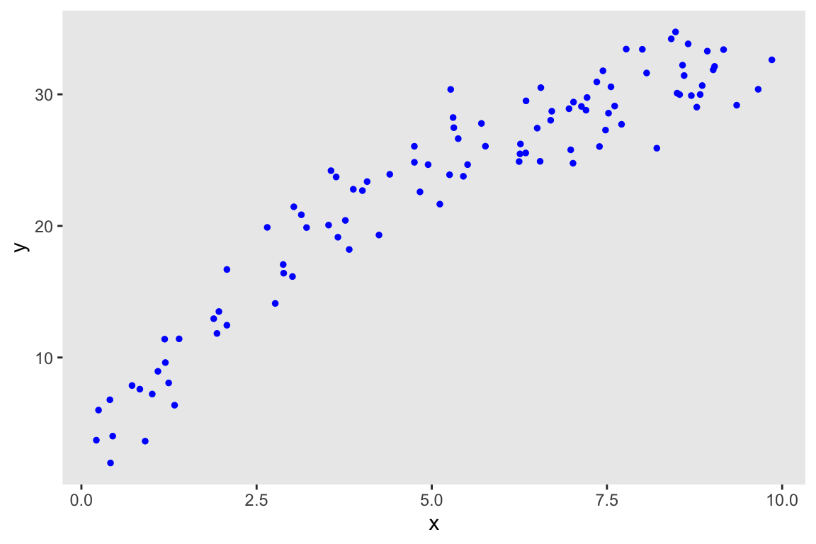
fit <- mod$sample(
  data = list(N = nrow(dd), x = dd$x, y = dd$y),
  seed = 72651,
  refresh = 0,
  chains = 4L,
  parallel_chains = 4L,
  iter_warmup = 500,
  iter_sampling = 2500
)
## Running MCMC with 4 parallel chains...
##
## Chain 1 finished in 0.1 seconds.
## Chain 2 finished in 0.1 seconds.
## Chain 3 finished in 0.1 seconds.
## Chain 4 finished in 0.1 seconds.
##
## All 4 chains finished successfully.
## Mean chain execution time: 0.1 seconds.
## Total execution time: 0.1 seconds.post_rvars <- as_draws_rvars(fit$draws())
x_rvar <- as_rvar(dd$x)
mu <- post_rvars$alpha + post_rvars$beta * x_rvar
pred <- rvar_rng(rnorm, nrow(dd), mu, post_rvars$sigma)
df.80 <- data.table(x = dd$x, y=dd$y, t(quantile(pred, c(0.10, 0.90))))
df.80[, extreme := !(y >= V1 & y <= V2)]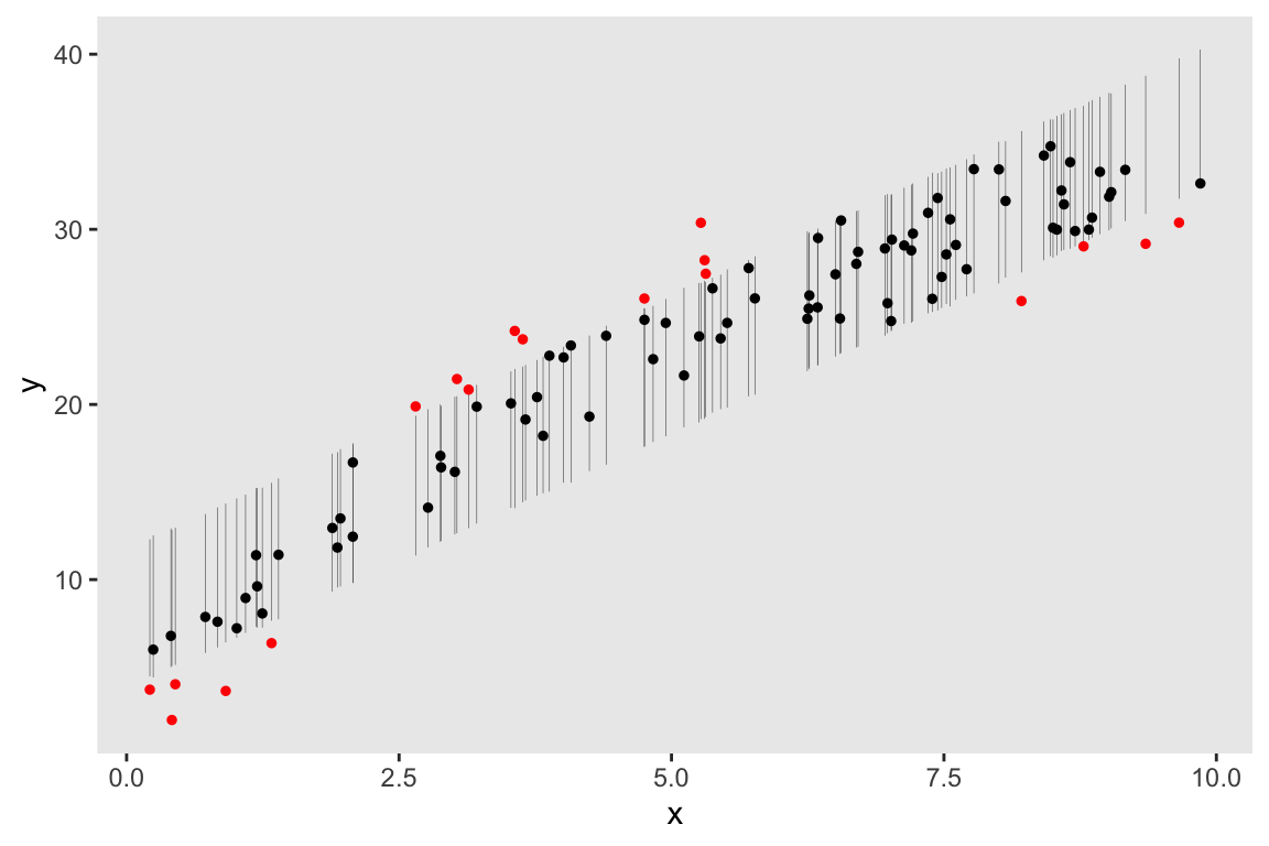
df <- data.frame(x = dd$x, y = dd$y, mu, pred)
df$grp <- cut(df$x, breaks = seq(0, 10, by = 2),include.lowest = TRUE, labels=FALSE)

bin_prop_y <- lapply(1:5, function(x) rvar_mean(with(df[df$grp == x,], (y < mu))))
array_y <- abind(lapply(bin_prop_y, function(x) as_draws_array(draws_of(x))))
rv_y <- rvar(array_y)

bin_prop_pred <- lapply(1:5, function(x) rvar_mean(with(df[df$grp == x,], (pred < mu))))
array_pred <- abind(lapply(bin_prop_pred, function(x) as_draws_array(draws_of(x))))
rv_pred <- rvar(array_pred)

(T_y <- rvar_var(rv_y))
## rvar<10000>[1] mean ± sd:
## [1] 0.11 ± 0.012(T_pred <- rvar_var(rv_pred))## rvar<10000>[1] mean ± sd:
## [1] 0.013 ± 0.0091mean(T_pred > T_y)## [1] 0I followed up this post with a quick update here.
References:
Gelman, Andrew. “A Bayesian formulation of exploratory data analysis and goodness‐of‐fit testing.” International Statistical Review 71, no. 2 (2003): 369-382.
Goldfeld, Stephen M., and Richard E. Quandt. “Some tests for homoscedasticity.” Journal of the American statistical Association 60, no. 310 (1965): 539-547.
Kerman, Jouni, and Andrew Gelman. “Manipulating and summarizing posterior simulations using random variable objects.” Statistics and Computing 17, no. 3 (2007): 235-244.