Estimating a risk difference (and confidence intervals) using logistic regression

Quickly defining the parameters of interest

In the study that motivated this, we had two study arms - an intervention arm which involved extensive outreach and vaccination promotion and the other a control arm where nothing special was done. So, there are two probabilities that we are interested in: \(p_1 \equiv P(\text{vaccinated} | \text{intervention})\) and \(p_0 \equiv P(\text{vaccinated} | \text{control}).\)

The risk difference comparing the two groups is simply

\[\text{RD} = p_1 - p_0,\] the odds \(w_a\) for each treatment group is

\[w_a = \frac{p_a}{1-p_a}, \ \ a \in \{0,1\},\] and the odds ratio comparing the intervention arm to the control arm is

\[\text{OR} = \frac{w_1}{w_0}.\]

The logistic regression model models the log odds as a linear function of the intervention status and any other covariates that are being adjusted. In the examples below, there is one continuous covariate \(x\) that ranges from -0.5 to 0.5:

\[\text{log}(w_A) = \alpha + \beta A + \gamma X.\] \(\beta\) represents the log(OR) conditional on a particular value of \(X\):

\[\text{log}(w_1) = \alpha + \beta + \gamma X \\ \text{log}(w_0) = \alpha + \gamma X, \] and

\[\text{log(OR)} = \text{log}\left(\frac{w_1}{w_0}\right) =\text{log}(w_1) - \text{log}(w_0) = \beta\]

More importantly, we can move between odds and probability relatively easily:

Estimating the marginal probability using model estimates

After fitting the model, we have estimates \(\hat{\alpha}\), \(\hat{\beta}\), and \(\hat{\gamma}\). We can generate a pair of odds for each individual \(i\) (\(w_{i1}\) and \(w_{i0}\)) using their observed \(x_i\) and the estimated parameters. All we need to do is set \(a=1\) and \(a=0\) to generate a predicted \(\hat{w}_{i1}\) and \(\hat{w}_{i0}\), respectively, for each individual. Note we do not pay attention to the actual treatment arm that the individual was randomized to:

\[ \text{log}(\hat{w}_{i1}) = \hat{\alpha} + \hat{\beta} + \hat{\gamma}x_i, \]

or

\[ \hat{w}_{i1} = \text{exp}(\hat{\alpha} + \hat{\beta} + \hat{\gamma}x_i). \]

Likewise,

\[ \hat{w}_{i0} = \text{exp}(\hat{\alpha} + \hat{\gamma}x_i). \] We get \(\hat{p}_{ia}\) for \(a \in \{0,1\}\) as

\[ \hat{p}_{ia} = \frac{1}{1 + \hat{w}_{ia}^{-1}}\]

Finally, the marginal risk difference \(\widehat{\text{RD}}\) can be estimated as

\[ \widehat{\text{RD}} = \frac{1}{n}\sum_{i=1}^n \hat{p}_{i1} - \frac{1}{n}\sum_{i=1}^n \hat{p}_{i0} \]

from all \(n\) study participants regardless of actual treatment assignment.

Fortunately, in R we don’t need to do any of these calculations as predictions on the probability scale can be extracted from the model fit. Standard errors of this risk difference can be estimated using bootstrap methods.

Simulated data set

Before getting into the simulations, here are the packages needed to run the code shown here:

set.seed(287362)

library(simstudy)
library(data.table)
library(ggplot2)
library(ggthemes)
library(parallel)

I am generating a binary outcome \(y\) that is a function of a continuous covariate \(x\) that ranges from -0.5 to 0.5. I use the beta distribution to generate \(x1\) which is transformed into \(x\). The advantage of this distribution is the flexibility we have in defining the shape. The OR used to generate the outcome is 2.5:

def <- defDataAdd(varname = "x1", formula = "..mu_x", variance = 8, dist = "beta")
def <- defDataAdd(def, varname = "x", formula = "x1 - 0.5", dist = "nonrandom")
def <- defDataAdd(def, varname = "y", 
  formula = "-2 + log(2.5) * rx + 1.5 * x",
  dist = "binary", link="logit")

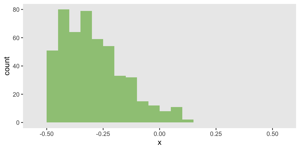
In the first scenario of 500 observations, the distribution of \(x\) will be right-skewed. This is established by setting the mean of \(x1\) close to 0:

mu_x = 0.2
  
dd_2 <- genData(500)
dd_2 <- trtAssign(dd_2, grpName = "rx")
dd_2 <- addColumns(def, dd_2)

ggplot(data = dd_2, aes(x = x)) +
  geom_histogram(fill="#9ec785", binwidth = 0.05, boundary = 0) +
  scale_x_continuous(limits = c(-.55, .55), breaks = seq(-.5, .5, by = .25)) +
  theme(panel.grid = element_blank())

The first step in estimating the risk difference is to fit a logistic regression model:

glmfit <- glm(y ~ rx + x, data = dd_2, family = "binomial")

Next, we need to predict the probability for each individual based on the model fit under each treatment condition. This will give us \(\hat{p}_{i1}\) and \(\hat{p}_{i0}\):

newdata <- dd_2[, .(rx=1, x)]
p1 <- mean(predict(glmfit, newdata, type = "response"))

newdata <- dd_2[, .(rx=0, x)]
p0 <- mean(predict(glmfit, newdata, type = "response"))

c(p1, p0)

## [1] 0.152 0.068

A simple calculation gives us the point estimate for the risk difference (and note that the estimated OR is close to 2.5, the value used to generate the data):

risk_diff <- p1 - p0
odds_ratio <- exp(coef(glmfit)["rx"])
  
c(rd = risk_diff, or = odds_ratio)

##    rd or.rx 
## 0.084 2.456

We can use a bootstrap method to estimate a 95% confidence interval for risk difference. This involves sampling ids from each treatment group with replacement, fitting a new logistic regression model, predicting probabilities, and calculating a the risk difference. This is repeated 999 times to get a distribution of risk differences, from which we extract an estimated confidence interval:

bootdif <- function(dd) {
  
  db <- dd[, .(id = sample(id, replace = TRUE)), keyby = rx]
  db <- merge(db[, id, rx], dd, by = c("id", "rx"))
  
  glmfit <- glm(y ~ rx + x, data = db, family = "binomial")

  newdata <- db[, .(rx=1, x)]
  p1 <- mean(predict(glmfit, newdata, type = "response"))

  newdata <- db[, .(rx=0, x)]
  p0 <- mean(predict(glmfit, newdata, type = "response"))

  return(p1 - p0)
}

bootest <- unlist(mclapply(1:999, function(x) bootdif(dd_2), mc.cores = 4))
quantile(bootest, c(0.025, 0.975))

##  2.5% 97.5% 
## 0.031 0.137

Change in distribution changes risk difference

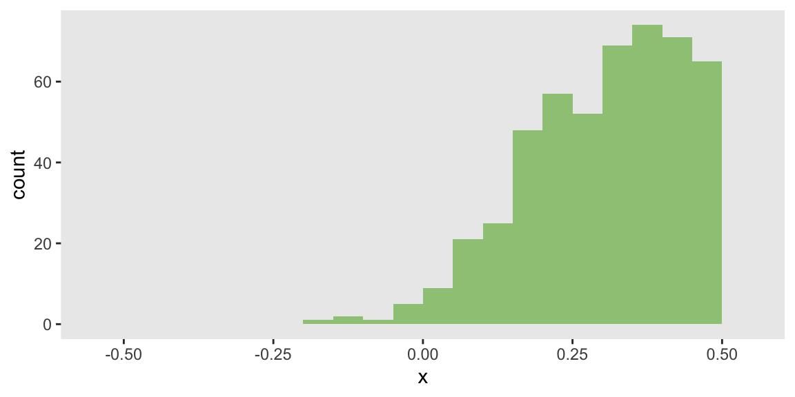
To illustrate how a shift in the distribution of \(x\) can influence the marginal risk difference without changing the odds ratio, I just need to specify the mean of \(x1\) to be closer to 1. This creates a left-skewed distribution that will increase the risk difference:

mu_x = 0.8

The risk difference appears to increase, but the OR seems to be pretty close to the true value of 2.5:

##    rd or.rx 
##  0.18  2.59

And for completeness, here is the estimated confidence interval:

##  2.5% 97.5% 
##  0.10  0.25

A more robust comparison

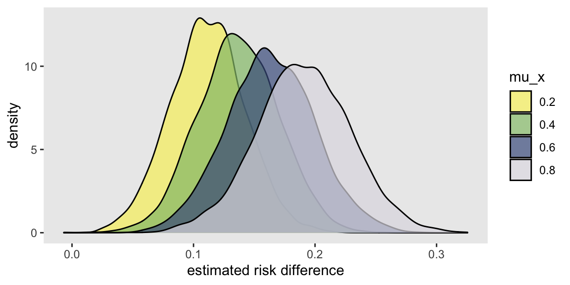
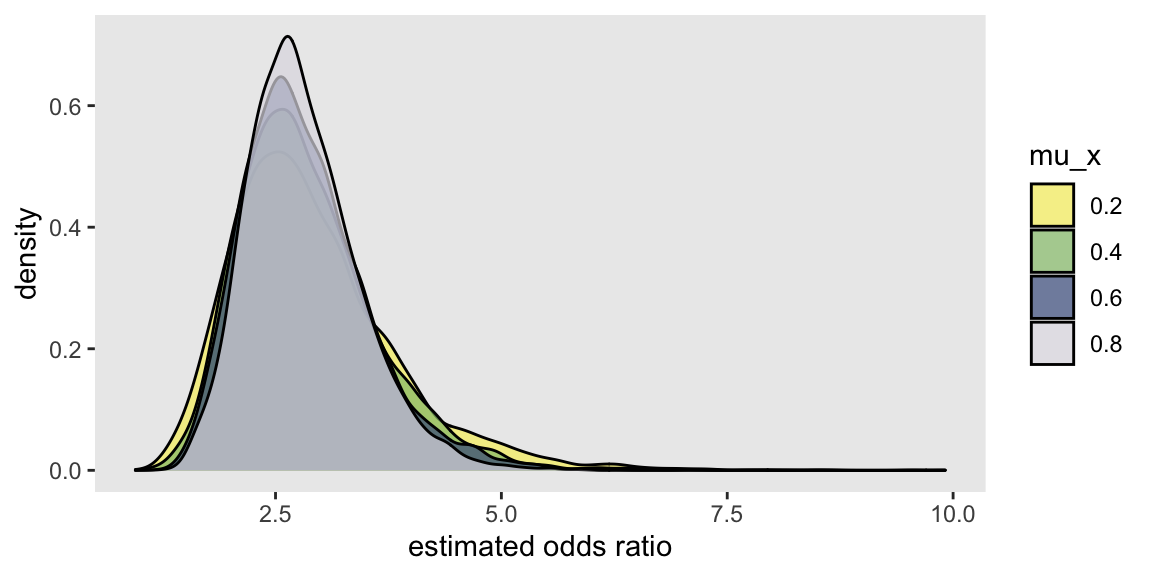
It is hardly fair to evaluate this property using only two data sets. It is certainly possible that the estimated risk differences are inconsistent just by chance. I have written some functions (provided below in the addendum) that facilitate the replication of numerous data sets created under different distribution assumptions to a generate a distribution of estimated risk differences (as well as a distribution of estimated ORs). I have generated 5000 data sets of 500 observations each under four different assumptions of mu_x used in the data generation process defined above: {0.2, 0.4, 0.6, 0.8}.

It is pretty apparent the the risk difference increases as the distribution of \(x\) shifts from right-skewed to left-skewed:

And it is equally apparent that shifting the distribution has no impact on the OR, which is consistent across different levels of \(x\):

Addendum: replication code

s_define <- function() {
  
  def <- defDataAdd(varname = "x1", formula = "..mu_x", variance = 8, dist = "beta")
  def <- defDataAdd(def, varname = "x", formula = "x1 - 0.5", dist = "nonrandom")
  def <- defDataAdd(def, varname = "y", 
    formula = "-2 + 1 * rx + 1.5 * x",
    dist = "binary", link="logit")
  
  return(list(def = def)) # list_of_defs is a list of simstudy data definitions
}

s_generate <- function(list_of_defs, argsvec) {
  
  list2env(list_of_defs, envir = environment())
  list2env(as.list(argsvec), envir = environment())
  
  dx <- genData(n)
  dx <- trtAssign(dx, grpName = "rx")
  dx <- addColumns(def, dx)
  
  return(dx) #  generated data is a data.table
}

s_model <- function(dx) {
  
  glmfit <- glm(y ~ rx + x, data = dx, family = "binomial")
  
  newdata <- dx[, .(rx=1, x)]
  p1 <- mean(predict(glmfit, newdata, type = "response"))
  
  newdata <- dx[, .(rx=0, x)]
  p0 <- mean(predict(glmfit, newdata, type = "response"))
  
  risk_diff <- p1 - p0
  odds_ratio <- exp(coef(glmfit)["rx"])
  
  model_results <- data.table(risk_diff, odds_ratio)
  
  return(model_results) # model_results is a data.table
}

s_single_rep <- function(list_of_defs, argsvec) {
  
  generated_data <- s_generate(list_of_defs, argsvec)
  model_results <- s_model(generated_data)
  
  return(model_results)
}


s_replicate <- function(argsvec, nsim) {
  
  list_of_defs <- s_define()
  
  model_results <- rbindlist(
    parallel::mclapply(
      X = 1 : nsim, 
      FUN = function(x) s_single_rep(list_of_defs, argsvec), 
      mc.cores = 4)
  )
  
  model_results <- cbind(t(argsvec), model_results)
  
  return(model_results) # summary_stats is a data.table
}

### Scenarios

scenario_list <- function(...) {
  argmat <- expand.grid(...)
  return(asplit(argmat, MARGIN = 1))
}

#----

n <- 500
mu_x <- c(0.2, 0.4, 0.6, 0.8)

scenarios <- scenario_list(n = n, mu_x = mu_x)

summary_stats <- rbindlist(lapply(scenarios, function(a) s_replicate(a, nsim = 5000)))

ggplot(data = summary_stats, aes(x = risk_diff, group = mu_x)) +
  geom_density(aes(fill = factor(mu_x)), alpha = .7) +
  scale_fill_canva(palette = "Simple but bold", name = "mu_x") +
  theme(panel.grid = element_blank()) +
  xlab("estimated risk difference")

ggplot(data = summary_stats, aes(x = odds_ratio, group = mu_x)) +
  geom_density(aes(fill = factor(mu_x)), alpha = .7) +
  scale_fill_canva(palette = "Simple but bold", name = "mu_x") +
  theme(panel.grid = element_blank()) +
  xlab("estimated odds ratio")

References:

Austin, Peter C. “Absolute risk reductions, relative risks, relative risk reductions, and numbers needed to treat can be obtained from a logistic regression model.” Journal of clinical epidemiology 63, no. 1 (2010): 2-6.
Kleinman, Lawrence C., and Edward C. Norton. “What’s the risk? A simple approach for estimating adjusted risk measures from nonlinear models including logistic regression.” Health services research 44, no. 1 (2009): 288-302.
Richardson, Thomas S., James M. Robins, and Linbo Wang. “On modeling and estimation for the relative risk and risk difference.” Journal of the American Statistical Association 112, no. 519 (2017): 1121-1130.
Support:
This work was supported in part by the National Institute on Aging (NIA) of the National Institutes of Health under Award Number U54AG063546, which funds the NIA IMbedded Pragmatic Alzheimer’s Disease and AD-Related Dementias Clinical Trials Collaboratory (NIA IMPACT Collaboratory). The author, a member of the Design and Statistics Core, was the sole writer of this blog post and has no conflicts. The content is solely the responsibility of the author and does not necessarily represent the official views of the National Institutes of Health.